Estimation of cumulative loss of strength of fittings for high temperature low sag overhead line conductors over their service life
AUTHORS
B. SOPPE, M. BENDIG, R. PUFFER - IAEW of RWTH Aachen University, Germany
H.J KRISPIN, M. DANSACHMÜLLER, S. ZEMKE - RIBE Elektroarmaturen GmbH, Germany

Summary
A new approach is presented to consider cumulative loss of strength of fittings for high temperature low sag conductors (HTLS conductors) over their service life. The loss of strength of an exemplary compression midspan joint made of aluminium alloy is estimated for various current and weather scenarios. At first, these current and weather scenarios, which may occur over the service life of the fitting, are defined. A validated thermal simulation model is used to determine fitting temperatures. Annual frequency distributions of fitting temperatures are obtained for the current and weather scenarios. A model to estimate cumulative loss of tensile strength is derived which is used to predict the residual strength of the fitting at the end of its design service life. The results show moderate loss of strength for most of the investigated weather regions and current profiles considered. It is proposed to use the approach to develop conditioning procedures in qualification tests of fittings.
Nomenclature
CDC Climate-Data-Center
CMSJ Compression mid-span joint
DWD Deutscher Wetterdienst (German institution for weather analysis)
HACIN High-strengthen aluminium-clad invar
HTLS High temperature low sag
MCOT Maximum continuous operating temperature
RCU Relative current utilization
RTU Relative thermal utilization
TSO Transmission system operator
UCTE Union for the Coordination of Transmission of Electricity
ZTAL Super thermal resistant aluminium
PJ,i Heat gain by Joule heating of finite element i
PS,i Heat gain by Solar heating of finite element i
PC,i Heat loss by convective heat dissipation of finite element i
Pr,i Heat loss by radiation of finite element i
PT,i Heat loss by conduction of finite element i
I Current
RDC,i DC Resistance
αi Absorption factor
Di Diameter of finite Element
dxi Length of finite Element
IB Direct solar radiation
Id Diffuse sky radiation
F Albedo
Hs Solar irradiation angle
η Angle of solar radiation to the conductor
EG Global radiation
εi Emissivity
σB Stefan-Boltzmann constant
Nui,90 Nusselt number for a perpendicular air flow
Nui,φ Nusselt number for an angle of attack φ
φ Angle of attack of the wind relative to the conductor
Rth,i Average thermal resistance of finite element i
AT,i Thermal conductive cross-section
κi Thermal conductivity
Resistance per unit length of CMSJ
Resistance per unit length of conductor
Transverse resistance of the contact
Rm (T,t) Tensile strength
Rm,init Initial tensile strength
rm Relative residual strength
erel Relative loss of tensile strength
Keywords
Fittings – HTLS conductor – loss of strength – overhead power lines – test recommendations1. Introduction
The increasing shift from traditional non-renewable energy sources towards renewable energy, brings about the necessity of transmitting electric energy from regions with an abundance of wind or solar generation (e.g., the coastal regions of northern Germany) to highly industrialized regions with an ample demand for energy (e.g., the south of Germany). This results in bottlenecks in the German transmission grid, which is largely consisting of overhead power lines. In Germany, measures to uprate the transmission capacity are prioritized according to the NOVA principle (network optimization before network reinforcement before network expansion). The use of high temperature low sag (HTLS) conductors is a reinforcement measure of the NOVA principle that can be used to uprate existing overhead power lines. These special conductors allow higher maximum continuous operating temperatures (MCOT) (> 200°C) and thus a higher ampacity compared to standard conductors (MCOT of 80 °C as per German design codes) with a comparable electrical conductive cross-section. However, the MCOTs of HTLS conductors lead to a higher thermal stress of fittings used to tension, connect and suspend the conductor which must be taken into account in the design process.
Aluminium alloys commonly used for conductor fittings have a material-specific temperature limit of about 90°C [1–3]. Above this temperature, unacceptable loss of tensile strength is expected [3, 4]. This limit temperature is much lower than the MCOT of the conductors with which the fittings will be used. Hence there is a need to consider the effect of operation at elevated temperatures on strength of fittings over their design life.
However, the effect of loss of tensile strength is cumulative over time and the conductor is not permanently operated at MCOT [5, 6]. The MCOT is only reached when the rated current of the conductor is flowing and a worst case weather situation (hot summer day) is present.
These conductor rating conditions occur only rarely (if at all) [7]. One approach to design fittings is to assume that the conductor constantly runs at MCOT and to size them large enough to keep their maximum temperature below 90 °C under the aforementioned rating conditions of the conductor. If the maximum temperature of the fitting stays below 80 °C one could even argue that testing according to IEC 61284:1997 might be adequate. However, keeping the maximum fitting temperature below 80 or 90°C may result in rather oversized fittings.
Another question is how to devise tests simulating thermal effects that might impair the strength of the fittings over their operating life.
A new approach developed within the funded project "FitTherm" is to consider the realistic temperature response of fittings for HTLS conductors to current loads and weather conditions. The proposed methodology takes into account the cumulative effect of temperature induced loss of tensile strength over the design lifespan of fittings and allows to predict residual strength. The same approach can be used to devise short-time tests that allow to simulate the expected loss of strength over the design life of the fitting.
First, different scenarios for the current load and weather conditions for Germany are explored and chosen for further consideration. Values characteristic for these scenario are used as input parameters for a steady state thermal simulation model to calculate the maximum temperature for the fitting under consideration. The resulting frequency distribution of occurring temperatures within the design lifespan are used to predict the fitting’s residual strength at the end of its design life. For that purpose, a model to calculate loss of tensile strength as a function of time and temperature of a commonly used aluminium alloy is introduced. Figure 1 summarizes the approach to estimate residual strength of fittings.
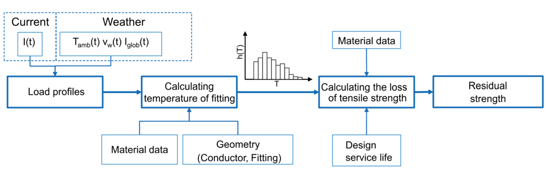
Figure 1
Scheme for calculating the residual strength of the fitting as a function of the current I(t), ambient temperature Tamb(t), wind speed Vw(t) and global radiation intensity Iglob(t)
In this paper the approach and results of the investigation is applied for an exemplary application consisting of a compression mid-span joint (CMSJ) in conjunction with a HTLS conductor consisting of an ultra-thermal resistant aluminium alloy conductor and an invar core (ZTAL/HACIN). The conductor is composed of two stranded core layers of High-strengthen Aluminium-Clad Invar (HACIN) with a cross-section of 34 mm² and two stranded layers of Super Thermal Resistant Aluminium (ZTAL) with a cross-section of 264 mm².
However, it should be mentioned that the presented method is applied to a variety of different fittings within the project “FitTherm”, including dead ends, suspension clamps and compression mid-span joints.
At first, the investigated scenarios are presented and necessary assumptions are discussed. Secondly, the model to calculate the maximum steady state temperature of the CMSJ and the model to calculate loss of tensile strength of the material is presented. Subsequently, resulting values of residual strength for the investigated scenarios are presented and discussed. Finally, thermal conditioning procedure is outlined that simulates the expected loss of tensile strength of fittings for HTLS conductors and could be used in qualification testing of fittings for HTLS conductors.
2. Scenario Definition
Load scenarios characterized by current and weather data are required to predict the temperatures of the CMSJ occurring over the years of operation. The weather data are taken from the Climate-Data-Center (CDC) of the DWD (Deutscher Wetterdienst, national weather service). The current data are obtained from various sources which are specified in the respective section below.
The design service life of overhead power lines is specified in the standard EN50341-1 as 50 years [8]. Accordingly, a design service life of 50 years is also assumed for the CMSJ and set as the scenario duration. However, the procedure can be applied using any other specified service life of choice. In addition, it should be noted that the design service life of the conductor used for the fitting is assumed to have the same design service life.
The approach presented in this paper allows for a decrease in tensile strength due to frequently occurring high temperatures. Therefore, it is necessary to define to what extent loss of strength of the material is considered permissible. The IEC 62004 standard for “Thermal-resistant aluminium alloy wire for overhead line conductor” is used as a guideline [9]. For the aluminium alloy of the ZTAL/HACIN conductor used in this paper, a residual tensile strength of 90 % of the initial tensile strength at the end of the design service life is considered acceptable. For this reason, the maximum permitted loss of tensile strength of the fittings aluminium alloy is defined as 10 %.
2.1. Definition of the weather scenarios
For the scenarios, weather data from the Climate-Data-Center (CDC) of the German national weather service are used. Weather data from about 400 weather stations are available in different temporal resolutions. This includes the ambient temperature, wind speed and global radiation. A maximum temporal resolution of 10 minutes is available for these variables, which is used for the weather scenario. In addition to the recorded weather data, metadata are available, with information on the geographical location, measuring instruments used, height of the measuring instruments above sea level and above ground level and quality of the measured data [10].
Weather conditions vary locally to a large extent. For this reason, a spatial division of Germany into 15 climate regions is used, in order to simplify the evaluation of the extensive weather data. These 15 climate regions were determined by the German weather service by means of cluster analysis in Germany. The analysis identified 15 clearly distinguishable regions, for each of which a weather station is representative [11].
For this paper, the weather years from 2010 to 2018 are considered. The year 2010 is chosen as starting year because the data basis for all necessary weather variables is consistent from this year on. It may be mentioned that the years considered, 2015, 2016, 2017, and 2018, are the hottest years globally since weather records began [12]. However, the 9-year period of the weather data used does not represent a statistically relevant period for considering the effects of climatic change, and it is not the intention of this paper to do so [13].
Missing data of wind speed and ambient temperature are replaced by linear interpolation except for the global radiation. Since no global radiation is present at night, a linear interpolation is not suitable. Instead, missing values of global radiations during the day are replaced by data from the previous year.
Since the overhead power line represents a spatially extended system and the wind along a line does not have a consistent angle of attack, a conservative estimate is made with regard to the angle of attack on the conductor and fitting. An angle of 25 ° is a recommended worst-case estimate especially for wind speeds below 2 m/s[14]. Additionally, wind speed increases with increasing height above ground, depending also on the surface roughness of the ground [14]. The wind speed at the 15 stations is measured on average at a height of approximately 15 m above the ground (minimum at10 m, maximum at 37.7 m). At voltage levels of 380 kV, minimum clearances of conductor to ground in Germany are in the range of 10 to 15 m. Therefore, the wind speeds measured by weather stations were directly used without correction for height above ground.
The weather stations measure the net global radiation (direct and indirect component), but not the component reflected by the ground (albedo). For this reason, the albedo is conservatively estimated to be 0.3 (for sand) [15]. Higher values for albedo may occur with ice and snow. However, although albedo is underestimated for these conditions resulting fitting temperatures are not expected to be critical because at the same time ambient temperatures usually will be low.
2.2. Definition of current scenarios
In order to calculate the relative frequency of fitting temperatures over a given year a current profile needs to be defined. Current profiles or scenarios were available from internal power flow simulations (PFS) performed at the IAEW of RWTH Aachen University and measured current values of TSOs. Additionally, defined constant current profiles were taken into consideration.
Available current values I are normalized to the rated current Irated of the conductor in order to derive a relative current utilization (RCU) of the line which is defined by (1).
(1)
With this RCU, the temperature calculation can be done for any conductor and is not specific to the used conductor type.
Joule heating is proportional to the square of the current. For this reason, current profiles are characterized by the integral of the squared current over one year or relative thermal utilization (RTU) which is defined by (2). For convenience, the current-square integral is normalized to the current-square integral of the rated current over one year.
(2)
The PFS data are based on power flow simulations of the transmission system that covers the network of the former “Union for the Coordination of Transmission of Electricity” (UCTE). The UCTE was a former administrative organization that has been taken over by the European Network of Transmission System Operators for Electricity (ENTSO-E) in 2009. However, the UCTE has administrated a synchronous network area in continental Europe which is modelled by the IAEW of RWTH Aachen. The conducted power flow simulations cover the voltage levels 220 kV and 380 kV in 2018.A total of 5714 load profiles from overhead power lines with a temporal resolution of 1 h are extracted. For these, redispatch measures were also taken into account during the simulation. From this extensive data set, one current profile is selected, which will be considered in this paper. The relative frequency of the RTU for all 5714 PFS profiles is shown in Figure 2. A maximum RTU value of 63 % can be found. Additionally, the 99 % quantile limit is shown. Below this limit 99 % of the RTU values of the 5714 PFS profiles can be found.
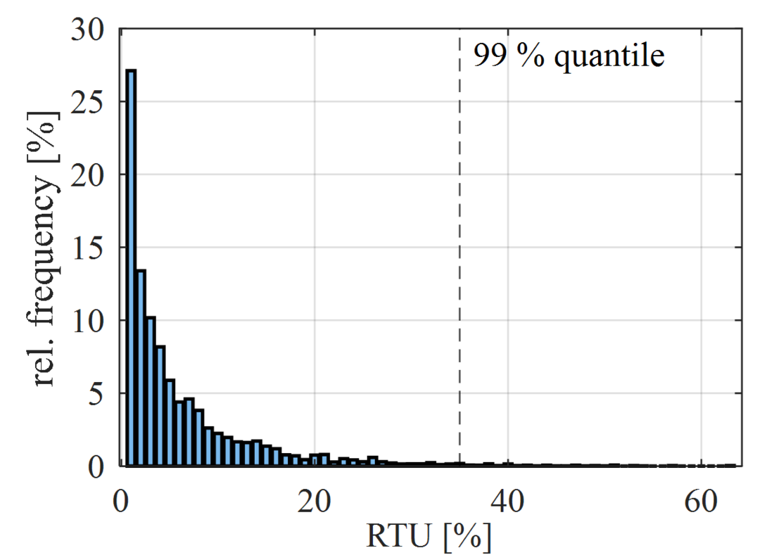
Figure 2 - Relative frequency of the relative thermal utilization of all 5.714 load profiles
A more detailed look at the relative frequencies of occurring relative RCU for the PFS profile with the highest RTU value is shown in Figure 3.
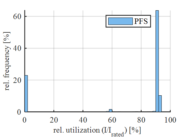
Figure 3 - Relative frequency of relative current utilization of the power flow simulation profile with the highest RTU
It can be seen that the RCU of the line is predominantly above 90 %. This profile is classified as unrealistic for HTLS conductors, since permanently high RCU rates cause high losses and this contradicts the actual application area of HTLS conductors. Instead, a PFS profile is selected which has a higher RTU value than 99 % of the PFS profiles (PFS99). The relative frequencies of occurring RCU for this profile is shown in Figure 4. The RCU ranges from over 40 % up to 80 % which on the one hand is considered to be a more realistic case for HTLS conductors and on the other hand a conservative profile.
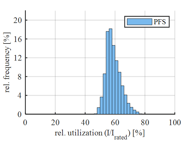
Figure 4 - Relative frequency of current utilization of the PFS profile with an RTU higher than 99 % of the other PFS profiles
From the measurement data of different TSOs, a profile is selected which originates from an overhead power line section on which HTLS conductors are installed. This profile was chosen to compare an actual HTLS overhead power line to the PFS profile. Compared to this profile, the PFS99 represents a highly utilized line. Figure 5 plots RCU versus relative frequency of occurrence for this profile.
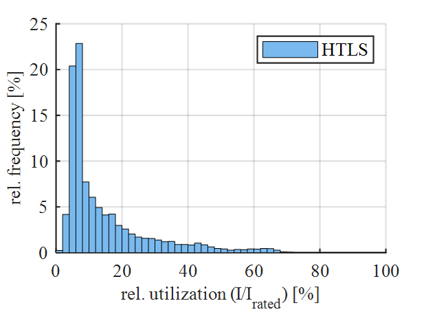
Figure 5 - Relative current utilization of the HTLS current profile
It can be seen that the frequency of high RCU is much more moderate compared to the PFS99 profile.
In addition, two reference scenarios are defined where a constant RCU of 75 % and 100 % of the conductor is assumed. The profile with 75 % RCU is called ‘Highly Utilized’ (HU) and serves as a reference scenario for the worst case when no (n-1)-case is present. The profile with 100 % RCU (RC) reflects the unrealistic case of current test recommendations, but linked to real weather scenarios.
All available current data has a lower temporal resolution than the weather data. Therefore, the current data are linearly interpolated and divided into 10 minute intervals.
Table I summarizes all the current profiles used for the investigations with their respective RTU. With these profiles, a good range of considered RTU is obtained.
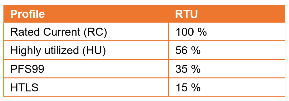
Table 1 - Relative thermal utilization (RTU) of used current profiles
2.3. Profile structure
For the temperature calculation of the CMSJ for a period of 50 years, a 9-year temperature profile is calculated for the weather years 2010 to 2018 with the different current scenarios. The 9-year temperature profile is assumed to recur and is repeated to form a length of 50 years. The last 5 years of the 50-year temperature profile are composed of weather data from 2010 to 2014. The profile structure is shown in Figure 6. For each 10 minute interval the steady state maximum temperature of the fitting is calculated. The calculation of the temperatures is presented in chapter 3.
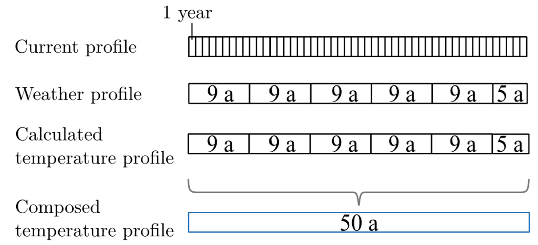
Figure 6 - Profile structure for the investigated scenarios
3. Simulation model
The calculation model for simulating the steady-state temperature distribution of conductor and fitting is based on the calculation rule from CIGRE's Technical Brochure 601 for conductors [15]. The model was chosen because it provides appropriate modeling capabilities for HTLS conductors [16]. The CIGRE model is modified in order to describe conductor and connected fittings. Conductor and fitting are divided into segments that differ in their geometry (effective cross-section, effective diameter), material properties and/or electrical/thermal characteristics. For example, the CMSJ is modelled by three segments, with two of the segments representing the compressed sections of overlap of the aluminium sleeve and conductor aluminium strands, respectively. The centre segment represents the section where there are no conductor aluminium strands beneath the aluminium sleeve. These segments are divided into finite elements of length and linked by a term describing the heat conduction between these elements. With respect to heat exchange with the environment, each finite element is modelled as a cylinder with a surface area equivalent to that of the original geometry. The same approach can be applied for all types of fittings (dead ends, suspension clamps etc.). The basic structure of the developed model is shown in Figure 7.
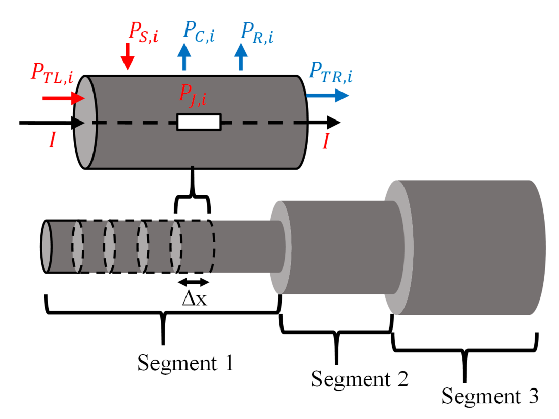
Figure 7 - Basic structure of the 1D model
The model was validated in the overhead line laboratory of the RWTH Aachen University in which the application of weather conditions (wind, ambient temperature, global radiation) as well as the current is possible [17].
The model uses the steady state heat balance (3) to calculate the temperature for a finite element i.
(3)
The individual power terms are heat transfer by convection PC,i and thermal radiation Pr,i, Joule heating PJ,i, heating by global radiation PS,i and heat transport by thermal conduction PT,i. The power transport by thermal conduction consists of the part PTL,i going into the element on the left and PTR,i going out of the element on the right. The power terms, except for heat transport by thermal conduction, are modeled according to the calculation rule for conductors in overhead power lines and are presented below [15].
Joule heating is calculated for each element according to (4), with current I and temperature dependent DC resistance .
(4)
Experiments conducted in the overhead line laboratory of RWTH Aachen University show that heating by DC compared to heating by AC causes a maximum relative temperature deviation of the absolute temperature below 1.3 % for the conductor with the CMSJ investigated in this paper. Due to many conservative assumptions made, the skin effect that becomes effective with alternating current is therefore neglected.
To calculate power input from global radiation (5) is used with absorptivity , diameter Di and length dxi of each element. IB, Id and F being direct solar radiation, diffuse sky radiation and albedo, respectively. With a solar irradiation angle (Hs) and an angle of solar radiation to the conductor (η) of 90°, (6) is derived. This is a worst case definition since the effect of radiation components is at a maximum. The global radiation EG includes direct and diffuse radiation IB and Id .
(5)
(6)
The equation to account for heat emission by heat radiation of each element i is given by (7). This equation includes diameter Di, emissivity and absolute surface temperature Ts,i of each element as well as the Stefan-Boltzmann constant
and absolute ambient temperature Ta.
(7)
With (8), convective cooling for each element is calculated using the thermal conductivity of air , surface temperature
, ambient temperature
and Nusselt Nui number.
(8)
The Nusselt number is calculated according to CIGRE TB601 with a rough surface, which results from round wires of the investigated conductor. The CMSJ has a smooth surface, thus the Nusselt number is calculated accordingly for a smooth cylinder. Additionally, the Nusselt number is corrected for the angle of attack between wind and conductor or fitting. The calculation rule according to CIGRE TB601 provides a model that is valid for Reynolds numbers < 4000 and makes the distinction between conductors with rough and smooth surfaces. The Reynolds number characterizes the flow properties of the wind and is used to calculate the Nusselt number at forced convection. For larger Reynolds numbers which result at higher wind speeds, the calculation of the correction factor for the angle of attack of the wind is done according to (9) [18]. The formula represents an approximation of discrete ratios of the Nusselt number at an angle of attack
and the Nusselt number for a perpendicular flow
, as a function of the angle of attack.
(9)
Heat transport by thermal conduction between elements is calculated with (10).
(10)
Heat flow results from temperature differences between adjacent elements and
divided by the average thermal resistance between adjacent elements. For each element, the thermal resistance is calculated using (11) with thermal conductive cross-section AT,i and thermal conductivity
.
(11)
An important physical characteristic is the electrical contact between conductor and fitting as applied in [19] for the CMSJ. Figure 8 schematically shows the contact area of the conductor and CMSJ. The model used is based on the circuit diagram in Figure 9 for a volume element of length dx.
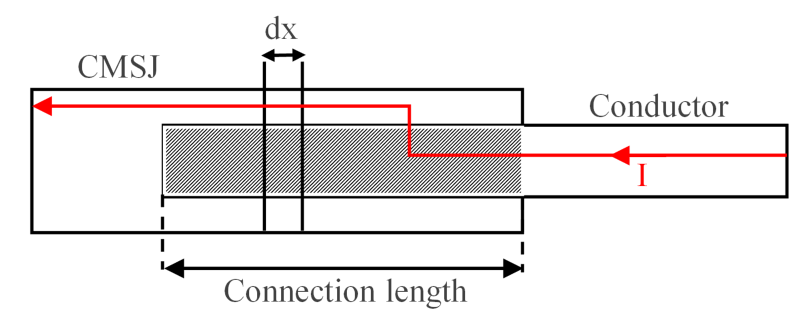
Figure 8 - Contact area of the CMSJ according to [19]
In the contact area, a current transfer from the conductor to the CMSJ takes place, which depends on the respective resistance per unit length of the contact partners and
and on the effective transverse resistance
in
. For each volume element in the contact area, all length and transverse resistances are assumed to be homogeneous.
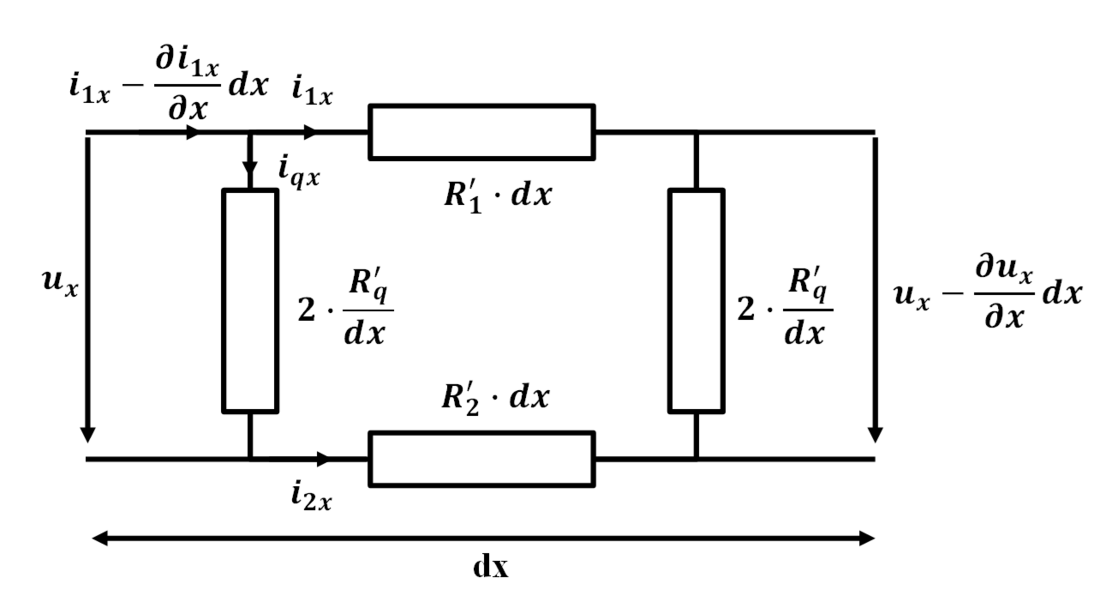
Figure 9 - Circuit diagram of a contact element of length dx according to [19]
For the CMSJ, the transverse resistance of is set to 0.2 µΩ∙m according to literature [19]. Contact aging is neglected in the context of this paper as it is assumed that design and installation of the CMSJ is such that the electrical contact remains stable [20].
The different expansion coefficients of the core and conductor material lead to a stronger temperature-related expansion of the conductor material (aluminium). This causes the aluminium layers to separate from the core layers of the conductor, which results in an increase in the conductor diameter and lower thermal coupling of the aluminium wires to each other. This effect is often referred in the literature to as bird-caging due to the visual appearance [21]. The increase in in diameter of the conductor with increasing temperatures leads to a higher heat dissipation by convection and radiation. At the same time, the thermal coupling between individual wires of the conductor leads to a reduced thermal conductivity in radial direction. In the simulation presented, the worst-case scenario is assumed in which the initial diameter of the conductor is set and a radial thermal conductivity of 0.7 W/(m*K) is used [15]. A radial thermal conductivity of 0.7 W/(m*K) assumes that the conductor is operated above the thermal transition point at which aluminium wires of the conductor are loose and the whole tensile force is on the core of the conductor. Thermal coupling between aluminium wires of the conductor is minimal above this operating point [16].
3.1. Definition of emissivities
The emissivity of a surface describes the amount of emitted thermal radiation in relation to an ideal radiator (black body). It can be in the range of 0.2 to 0.3 for new conductors. Depending on the years of service and environment, the emissivity can increase up to 0.9 [14, 22].
For the investigated scenarios emissivity is set to 0.55 which is considered to be a conservative estimate for a conductor after several years of service and is often stated in datasheets of conductor manufacturers. It is assumed that the deposits on the conductor and fitting are uniform and therefore emissivity is the same for conductor and fitting. The absorption factor is assumed to be 0.1 higher than emissivity [15, 16]. Since the emission factor for new conductors is lower than the specified 0.55, it is assumed that higher loss of strength may occur in the first years due to higher possible temperatures. However, since the emission factor is expected to be above 0.55 for the majority of the service life of the fitting and conductor, it is assumed that the resulting lower temperatures will in turn lead to lower loss of strength.
4. Model to calculate loss of tensile strength
Aluminium-magnesium-silicon (AlMgSi) alloys are often used for fittings because of their high corrosion resistance, good workability, economic aspects and a good compromise between electrical conductivity, weight and strength. For the CMSJ, an AlMgSi alloy is used with the standard designation EN AW-6082 and composition according to EN 573-3 [23]. To increase the strength of aluminium and aluminium alloys, strain hardening and precipitation hardening is used. Due to the material treatment, dislocations are created in the microstructure causing an increase in tensile strength. This established strength of the material can be permanently degraded by a recovery process due to heat exposure which leads to a reduction of dislocations. For EN AW-6082, the so-called annealing curves are shown in Figure 10. The annealing curves show the tensile strength at ambient conditions as a function of exposure time to elevated temperatures. It can be seen that the decrease in tensile strength depends on temperature in a non-linear manner.
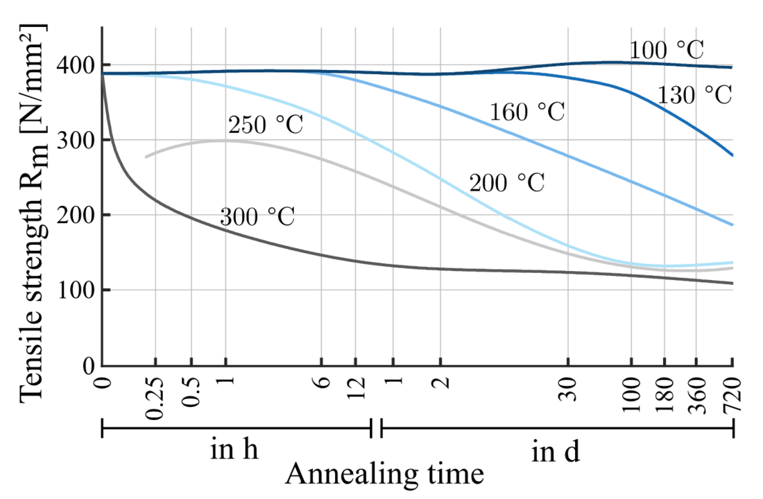
Figure 10 - Tensile strength curves of aluminium alloy EN AW-6082 for different annealing temperatures according to [6]
In order to derive the model equations to determine the loss of tensile strength of the material, the relative residual strength rm is defined as the ratio of temperature dependend tensile strength Rm(T) to initial tensile strength Rm,init (12).
(12)
If the annealing time and temperature for a certain Rm are taken from the diagram in Figure 10, an Arrhenius diagram can be obtained (Figure 11). On the ordinate the annealing time in h is plotted in base 10 logarithmic scale. The abscissa is the annealing temperature in 1000/K. In addition, two different curve fittings are shown. It can be seen that with a linear curve fitting, there is an overestimation of the time to reach a relative residual strength for the data points at 160 °C. Therefore, due to the limited data availability, a quadratic fit is used for the temperature range 130 °C – 200 °C as a conservative estimate regarding the annealing time and annealing temperature compared to a linear fit. For temperatures below 130 °C, the extrapolation of the linear fitting curve for the relative residual strength is used, which again represents a conservative estimate compared to the quadratic approximation for temperatures below 130 °C.
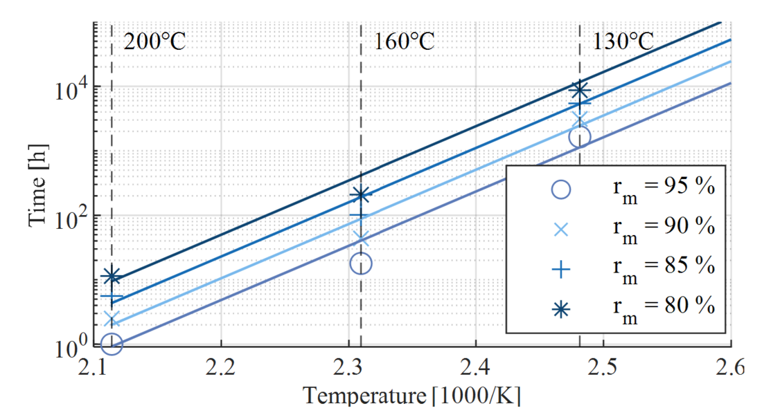
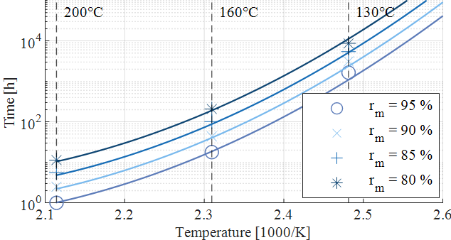
Figure 11 - Arrhenius diagram of the aluminium alloy EN AW-6082 for different annealing temperatures and a linear fit (left) and a quadratic fit (right)
The functional dependence of time t(rm,T) until degradation to a relative residual strength rm occurs is derived from the linear and quadratic curve fitting and is given by (13).
(13)
The determined constants for the EN AW-6082 alloy are shown in Table II.
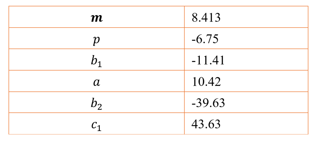
Table 2 - Constants for (13) of the EN AW-6082 alloy
To calculate the cumulative loss of tensile strength over the service lifespan of the fitting, the rate of degradation is required. This indicates the rate at which EN AW-6082 loses tensile strength as a function of temperature. For this purpose, the relative loss of tensile strength erel is introduced with (14).
(14)
It is assumed that the relative loss of tensile strength so obtained is characteristic for the overall loss of strength of the fitting under investigation. The rate of relative loss of tensile strength in (15) is obtained by substituting rm in (13) with (14), solving the equation for erel and differentiate (13) with respect to time.
(15)
According to the derived model, a permanent temperature of at least 81.32 °C is required to cause 1 % reduction in tensile strength after 50 years. Since the rate of loss of tensile strength is strongly nonlinearly dependent on temperature a permanent temperature of 90 °C leads to a loss of tensile strength of approx. 10 % after 50 years.
5. Residual strength for different scenarios
5.1. Residual strength at different climatic locations
The constant profile HU is used to compare rm at different considered climatic regions. Figure 12 shows a box-plot of the calculated fitting temperatures of all weather stations from 2010 to 2018. The temperature median values occurring at individual weather stations are shown in red. The boundaries of the blue boxes are defined by the quartiles. Furthermore, for each weather station the maximum and minimum value is shown. It can be seen that the median values of determined temperatures are in a moderate range. With a median maximum of just over 60 °C for the CMSJ at weather station 15, they are well below 81.32 °C at which significant loss of tensile strength can occur at all. However, the maximum values for each weather station clearly exceed 100 °C in all cases.
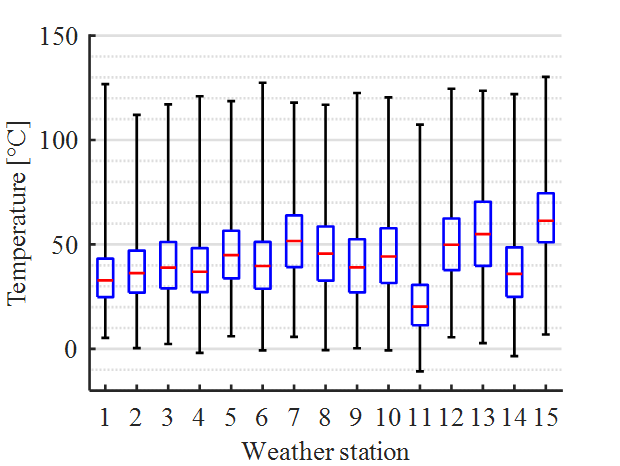
Figure 12 - Temperature of the CMSJ for all weather stations and HU current profile
In Figure 13, the calculated rm values based on the temperature data from Figure 12 are shown. For the data of all weather stations and the HU current profile, previously defined requirement of a minimum of 90 % of the initial strength is achieved. In particular, the loss of tensile strength at weather station 15 is the highest compared to the other weather stations.
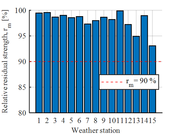
Figure 13 - Calculated relative residual strength for all weather stations and HU current profile
Reasons for lower rm values at weather station 15 can be explained by observing the wind speeds recorded at the individual weather stations. Figure 14 shows the relative frequency of occurring wind speeds at weather station 11 and 15. Weather station 11 is selected since the lowest loss of tensile strength is observed here. It can be seen that the relative frequency of wind speeds at weather stations 11 and 15 show a clearly different distribution. High wind speeds at weather station 11 are more frequent than those at weather station 15. The relative frequency of wind speeds from the other weather stations are between these two extreme distributions. For this reason, the higher loss of tensile strength at weather station 15 compared to all other weather stations can be attributed to the high frequency of low wind speeds. Therefore, only weather station 15 is considered in further analysis for the comparison between individual current profiles, since it represents the worst case with respect to wind speed and fitting temperature compared to other weather stations.
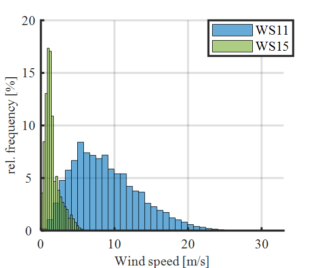
Figure 14 - Frequency of wind speeds at weather stations 11 and 15
5.2. Residual strength for different current profiles
The calculated temperatures for the different current profiles with the weather data from weather station 15 are shown in Figure 15. As with the HU profile, moderate median values of the occurring temperatures can be seen for the HTLS and PFS99 profiles. As expected, the reference profile RC shows the highest median value of calculated temperatures as well as the highest maximum value.
Although the RTU value of the HTLS profile is lower than of the PFS99 profile, the HTLS profile shows a slightly higher maximum temperature value of the fitting. The lowest temperature value for the HTLS profile can be seen for a winter day in 2012 with an ambient temperature of -22.2 °C. At the same time, RCU is 2.2 %.
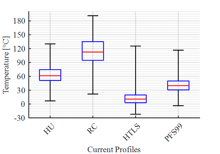
Figure 15 - Distribution of maximum temperature of the CMSJ for the current profiles from Table I using data from weather station 15
Resulting rm values of calculated temperatures in Figure 15 are shown in Figure 16. The HTLS profile leads to a slightly higher loss of tensile strength than the PFS99 profile. The strong nonlinearity of the model to calculate the loss of tensile strength is noticeable here. Temperatures for HTLS and PFS99 profiles are below the 130 °C limit where the linear approximation in (13) is used. Profiles PFS99 and HTLS both show hardly any loss of tensile strength.
The reference profile RC, on the other hand, shows a very high loss of tensile strength of almost 58 %.
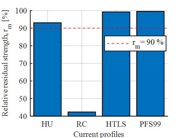
Figure 16 - Calculated relative residual strength for weather station 15 and different current profiles
6. Conclusion and outlook
The presented approach comprising definition of current load and weather scenarios, thermal simulation and modelling of cumulative loss of strength offers a way to predict residual strength of fittings for HTLS conductors at the end of their design life. Necessary simplifications and choice of parameters were made on the safe side. One of the simplifications consisted in assuming that the fittings are at steady state temperature at all times, thereby neglecting the thermal inertia of conductor and fitting.
The relative loss of tensile strength was found to be moderate for the investigated exemplary combination of conductor and CMSJ for the studied current profiles HU, HTLS and PFS99 in the weather region with the lowest measured wind speeds in Germany (weather station 15). Only the reference current profile RC shows an unacceptable degree of loss of tensile strength with the data from weather station 15. However, the reference current profile RC represents an unrealistic worst-case estimate. For the HTLS current profile, which represents a real current profile of an overhead power line stranded with HTLS conductors, the expected loss of strength is largely within acceptable limits.
The temperature of conductor and fitting depends on the geometry and electrical characteristics. Therefore, a consideration of the respective temperatures must be made for each type of fitting and conductor for the presented scenarios. Additionally, temperature activated loss of strength is known to occur for fittings which receive their strength from strain hardening as for example the aluminium sleeves of compression fittings or from precipitation hardening as for example forged suspension clamps made of AlMgSi aluminium alloys. For each kind of temperature activated loss of strength, a formulation based on the Arrhenius law can be found and needs to be introduced into the algorithm. The presented algorithm lends itself to predict different loss of strength, depending on different utilization of a line. The current profiles used in this paper to represent utilization of the line is deemed to be conservative, at least the PFS99 profile.
The presented algorithm also lends itself to assess the design of fittings with regard to their longtime mechanical strength under a chosen utilization of a line as the fitting's geometry is taken into account in the thermal simulation and the fitting's material is taken into account in the modeling of the loss of strength.
Furthermore, as the presented approach allows to estimate temperature induced loss of strength for any given set of current load and ambient conditions, it can be used to define a conditioning regime for a fitting. For a given relative residual strength, e. g. the one predicted for the fitting’s application, a temperature can be determined via the Arrhenius diagram in Figure 11 that results in the same relative residual strength, but within a significantly shorter time suitable for testing purposes. This temperature can be used in industrial laboratories for conditioning fittings for HTLS conductors. Here, the fitting temperature and not the conductor temperature is the reference variable. After the fitting has been conditioned, standard mechanical tests, e. g. as specified in IEC 61284, can be performed on the artificially aged fitting to prove its long-term reliability.
Future studies will address conditioning rules for fittings for HTLS conductors which need to be independent on fitting materials.
Acknowledgment
The authors thank Mr. Max Ole Christiansen for his contributions to this study.
The work presented in this paper was funded by the Federal Ministry of Economic Affairs and Energy as projects 0350006A and 0350006B.
References
- CIGRE WG B2.48, Experience with the mechanical performance of non-conventional conductors, Paris, CIGRÉ, 2017.
- VDE|FNN, Einsatz von Hochtemperaturleitern, Berlin, Forum Netztechnik/Netzbetrieb im VDE, 2013.
- CIGRE WG B2.26, Guide for Qualifying High Temperature Conductors for Use on Overhead Transmission Lines, Paris, CIGRÉ, 2010.
- J. Bodner, M. Höfer, M. Laußegger, G. Stampfer, H. Strobl und H. Wörle, “Use of high thermal limit conduc-tors in the replacement of 220 kV overhead lines in the Tirolean Alps”, CIGRÉ Session 2012, 2012.
- CIGRE WG B2.55, Conductors for the uprating of existing overhead lines, Paris, CIGRÉ, 2019.
- C. Kammer, Aluminium Taschenbuch 1: Grundlagen und Werkstoffe, 16. Aufl., Düsseldorf, Aluminium-Verl., 2009.
- R. Puffer, T. Frehn, M. V. Fonder, J. T. Krapp und M. Riedl, “220-kV field study of different high temperature low sag conductors”, CIGRÉ Session 2014, 2014.
- Overhead electrical lines exceeding AC 1 kV - Part 1: General requirements - Common specifications; German version EN50341-1:2012, Deutsche Norm 50341-1, 2013.
- Thermal-resistant aluminium alloy wire for overhead line conductor, Deutsche Norm 62004, 2010.
- DWD Deutscher Wetterdienst, Readme_intro_CDC_ftp.pdf. Available at: https://opendata.dwd.de/climate_environment/CDC/Readme_intro_CDC_ftp.pdf (29.03.2021).
- DWD Deutscher Wetterdienst und BBR, “Handbuch - Testreferenzjahre von Deutschland für mittlere, extreme und zukünftige Witterungsverhältnisse”, Offenbach, 2014.
- Agora Energiewende & Agora Verkehrswende, “15 Eckpunkte für das Klimaschutzgesetz”, 2019.
- IPCC Intergovernmental Panel on Climate Change, Climate change 2013: The physical science basis : Working Group I contribution to the Fifth assessment report of the Intergovernmental Panel on Climate Change, Cam-bridge, Cambridge University Press, 2014.
- CIGRE WG B2.12, Guide for Selection of Weather Parameters for Bare Overhead Conductor Ratings, Paris, CIGRE, 2006.
- CIGRE WG B2.43, Guide for thermal rating calculations of overhead lines, Paris, CIGRÉ, 2014.
- T. Frehn, “Thermische Modellierung von Hochtemperaturleitern für Freileitungen”, Dissertation, RWTH, Aachen, 2017.
- B. Soppe, T. Frehn, R. Puffer, H.-J. Krispin, M. Dansachmüller und S. Zemke, “Thermal modelling of fittings for high temperature low sag conductors”, VDE Hochspannungstechnik, 2020.
- I. Berg, “Untersuchungen zur Strombelastbarkeit der Geräte der Elektroenergieübertragung unter Freiluftat-mosphäre”, Dissertation, Institut für Elektrische Energieversorgungstechnik (IEEH), Technische Universität Dresden, Dresden, 2011.
- C. Hildmann, “Zum elektrischen Kontakt- und Langzeitverhalten von Pressverbindungen mit konventionellen und Hochtemperatur-Leiterseilen mit geringem Durchhang”, Dissertation, TU Dresden, Dresden, 2016.
- Overhead lines - Requirements and tests for fittings, IEC 61284, 1997.
- T. Frehn, R. Puffer, M. V. Fonder und M. Riedl, “Verification of thermal rating calculations for high tempera-ture low sag (HTLS) conductors”, CIGRÉ Session 2016, 2016.
- W. S. Rigdon, H. E. House, R. J. Grosh und W. B. Cottingham, “Emissivity of Weathered Conductors After Service in Rual and Industrial Environments”, Transactions of the American Institute of Electrical Engineers. Part III: Power Apparatus and Systems, 1962.
- Aluminium and aluminium alloys - Chemical composition and form of wrought products EN 573-3, 2019.