Generalized Approach to Analytical Circuit Breaker Transient Recovery Voltage Calculation
AUTHORS
D.F. PEELO - Independant Consultant

Summary
With the widespread availability of transient simulation software, the analytical calculation of circuit breaker transient recovery voltages (TRV) has tended to become a lost science. Part of the reason for this is the wide range of cases to be covered from terminal faults to load current switching. An examination of the circuits involved in the different current interruption cases shows a clear mathematical commonality in the equations describing the associated TRVs. This commonality allows a generalized approach based on circuit damping and oscillation angular frequency enabling TRV calculation and plotting using MS Excel. The derivation of the approach is explained and is fully supported by application of its use in real cases.
KEYWORDS
Circuit breakers - series reactors - shunt reactor switching - surge capacitors - terminal faults - transient recovery voltages1. Introduction
The intent of this paper is to describe the derivation of a generalized analytical approach to circuit breaker transient recovery voltage (TRV) calculation and to show how it can be used in real application cases. The notion of the approach is not new and has been attempted earlier but not without a false assumption [1], [2]. The approach and the assumption is discussed in the following.
The basic circuits involved are either a parallel or series RLC circuit. The damping in the circuit is determined by the value of R. Generalized damping requires that R be referenced in such a way that damping is unitized and becomes expressible as a per-unit quantity (the well-known amplitude factor kaf found in the standards). In reference [1], this is achieved by referencing R to the circuit surge impedance , the degree of damping being R/Z for a parallel RLC circuit. This is valid but leads to quite convoluted equations which are difficult to use. The false assumption in the approach is to create a claim of duality between series and parallel circuits whereby an equation derived for a parallel circuit is applicable to a series circuit simply by inverting the degree of damping, i.e. substituting Z/R for R/Z. There is a real duality between series and parallel circuits and it is discussed later. The equations were derived using Laplace transforms and the generic curves as are provided are correct but no attempt is made to demonstrate how the equations and curves can be used in practical reality.
An alternative basis for general circuit damping treatment was proposed, but not further developed, in a paper from 1951 [3]. The proposal is that the circuit resistance R be referenced in general to the resistance that results in critical damping and designated as Rc. The coefficient of damping is thus R/Rc or Rc/R depending on whether the circuit is series or parallel connected. The generalized equations and associated curves are derived on this basis in the following.
2. Generalized Equation Derivation
The approach exploits the fact that the different circuit cases have a common differential equation solution as shown in Table I. Three cases are shown in the table as follows:
- The first two rows show the cases and the associated circuits for calculation.
- The next two rows give the boundary conditions and the differential equations applicable to the case.
- Circuit damping calculation is given in the next row followed by three rows giving the solutions for each case based on the general solution in Table II in the Appendix and applying the boundary conditions.
- The last row lists the potential uses for the derived equations.
By way of example, taking the first series RLC circuit from Table I and with reference to the Appendix, the solution for the overdamped case is
where v is the voltage on the capacitor. Applying the boundary conditions gives the new equation
(1)
which is in per-unit and valid for real time and specific values of and
. To generalize the equation,
,
and t must be converted to generic values.
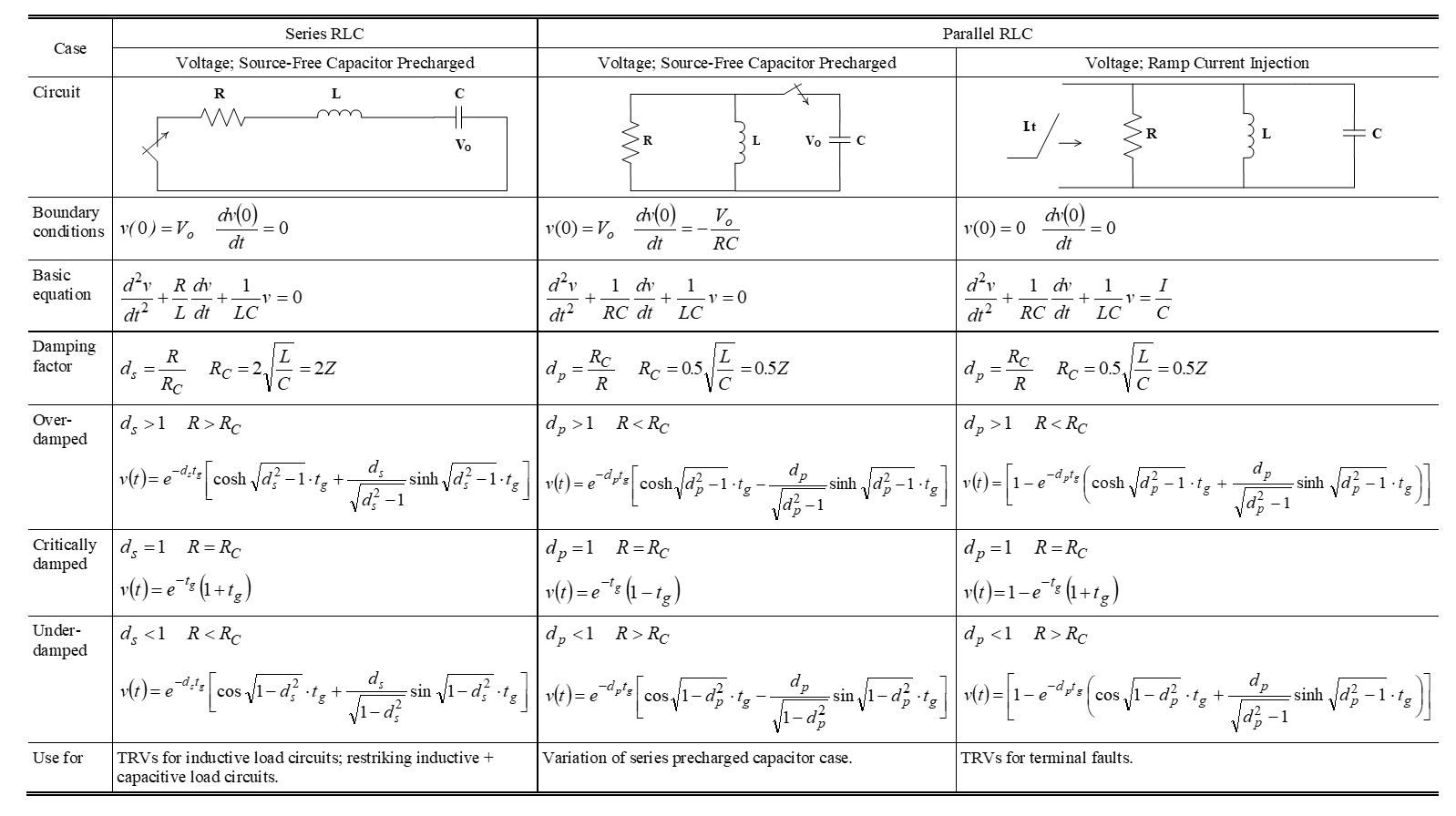
Table I - Series and Parallel Circuit Equations
From the Appendix and Table I the a, b and c values are
giving
and
where is the angular frequency in radians/second. For critical damping
and the corresponding resistance Rc is derived as follows
The degree of damping ds is defined as
meaning that circuit damping is referenced to critical damping as noted above.
Generic time tg, i.e. expressing time on a frequency basis, is given by dividing real time t by one period of the undamped angular frequency .
and (1) can be rewritten in the generic form shown in the table. Generalized damping curves for this case are plotted in Fig. 1.
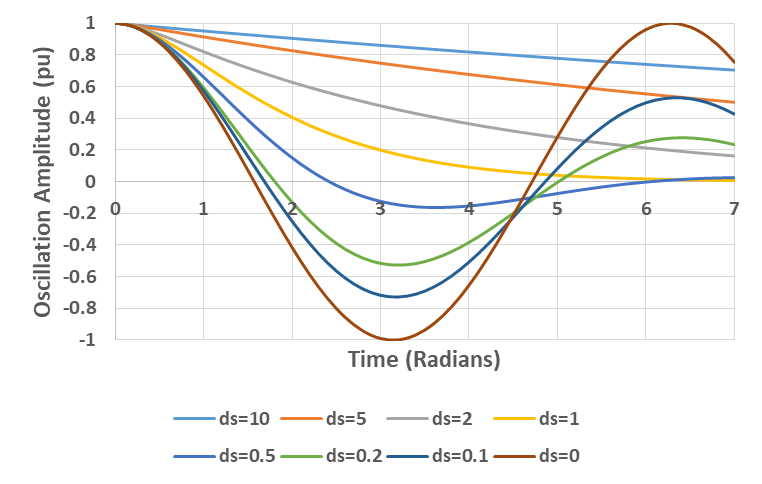
Figure 1 - Generalized damping curves for series RLC circuit with a precharged capacitor
By comparison to the parameters and equations for the parallel RLC circuit with a precharged capacitor, no obvious duality exists between the two cases.
With reference to the Appendix, the equation calculation for the parallel RLC ramp current injection case is similar to that for the above case. Generalized damping curves are shown in Fig. 2, noting that the curves now oscillate the 1 pu value.
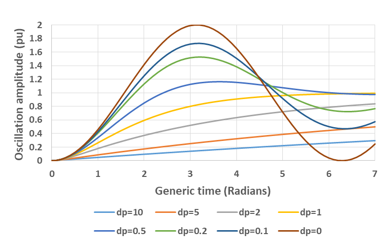
Figure 2 - Generalized damping curves for parallel RLC circuits with ramp current injection
Comparison of the equations shows that there is a duality between the series RLC circuit with a precharged capacitor and the parallel RLC circuit with ramp current injection. Likewise the same is true if the former is a parallel RLC circuit and the latter a series RLC circuit with ramp current injection [4].
3. Practical Examples
To illustrate the practical use of the approach the following examples will be considered: terminal fault and shunt reactor switching TRVs and generator circuit breaker TRVs with the addition of surge capacitors.
3.1 245 kV Circuit Breaker T30 TRV
The now-harmonized standard T30 TRV (30% terminal fault) requirements for a 245 kV circuit breaker are:
- Peak value uc = 400 kV.
- Rise time value t3 = 80 µs.
- Pole factor kpp = 1.3 pu.
- Amplitude factor kaf = 1.54 pu.
With reference to Fig. 2, 1 pu on the oscillation vertical axis is the peak value of the recovery voltage and equals 260 kV for the pole factor of 1.3 pu. For the horizontal axis 1 pu tg is derived from the t3 value and the time to peak T [4], [5]:
The remaining quantity to be determined is dp which is related to kaf as given in [4] and, for kaf = 1.54 pu, dp = 0.196 pu. The T30 TRV is therefore
The per-unit version of the equation (term inside the square brackets) is plotted in Fig. 3 (peak of 1.54 pu at radians as expected) and the real voltage and time in Fig. 4 (peak of 400 kV at 95 µs as expected).
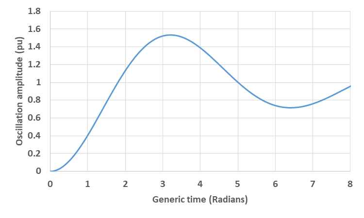
Figure 3 - 245 kV circuit breaker T30 TRV in per-unit voltage versus generic time
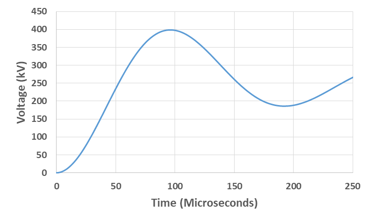
Figure 4 - 245 kV circuit breaker T30 TRV in real voltage versus real time
3.2 Shunt Reactor Switching
For shunt reactor switching the TRV is the difference between the power frequency source voltage on one side of the circuit breaker and the oscillation ring down voltage on the reactor side. The reactor is represented by a series RLC circuit and the ring down oscillation is underdamped with an amplitude factor kaf = 1.9 pu. The general per-unit equation for the TRV is
where K is the neutral shift, ka is the suppression peak, ds is the degree of damping and tg is generic time [4], [5]. For kaf = 1.9 pu, ds = 0.033 and the equation becomes
With a view to illustrating the calculation, take the case of a 516 kV, 135 Mvar reactor with its neutral point grounded through a neutral reactor giving K = 0.3 and a ka value of 1.229 pu. The generic equation for the case is
(2)
and 1 pu tg multiplier is 111 µs.
The Excel calculation is shown in Fig. 5 and is plotted in Fig. 6. Note that having the neutral reactor adds 0.6 pu to the TRV peak value and a good practice is to bypass the neutral reactor with a single pole disconnect switch prior to switching out the main reactor.
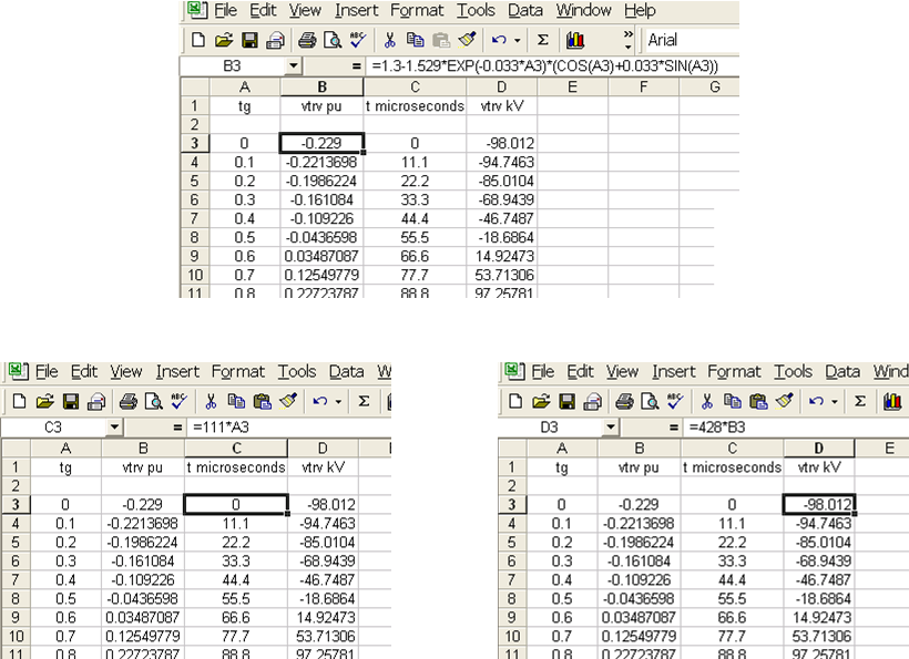
Figure 5 - Excel calculation illustration for Eqn (2)
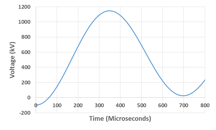
Figure 6 - Plot of TRV for the case calculated in Fig. 5
A frequently-asked question is whether the above shunt reactor considerations can be applied to series reactor applications? The answer is affirmative with due adjustment to the source side contribution now being a TRV rather than a power frequency one per-unit recovery voltage [4]. The starting point of each side TRV will be at the voltage drop on the reactor at the instant of current interruption and the circuit breaker TRV will be the difference between the source and load side TRVs. An example of such a calculation result is shown in Fig. 7. The calculation can be done with the reactor on the source side of the circuit breaker yielding the same result but the easiest approach is that described above [4].
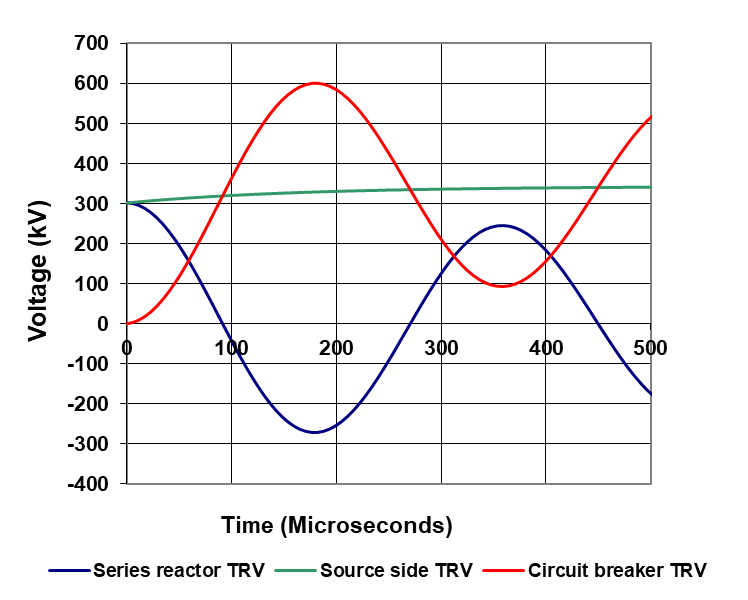
Figure 7 - Example of the result for a series reactor application circuit breaker TRV
3.3 Generator Circuit Breakers
For generator circuit breakers, the pole and amplitude factors are taken at 1.5 pu and the t3 and uc values are variable by the generator rating and the rated voltage of the circuit breaker [7]. The applicable TRVs are all underdamped and are those associated with system-source faults, generator-source faults, out-of-phase switching and load current switching.
By way of example, take the case of a 17.5 kV, 8000 A, 60 Hz circuit breaker with a system-source fault rating of 100 kA. From the standard:
- t3 = 0.46 Ur = 8.05 µs where Ur = 17.5 kV.
- uc = 1.82 Ur = 32.2 kV.
- kaf = 1.5 pu → dp = 0.215.
- kaf = 1.5 pu → T = t3/0.837 → 1 pu tg = 3 µs.
The TRV is represented by a parallel oscillatory RLC oscillatory circuit with L = 0.4 mH, C = 23 nF and R = 306 and given by the equation
and is shown plotted in Fig. 8.
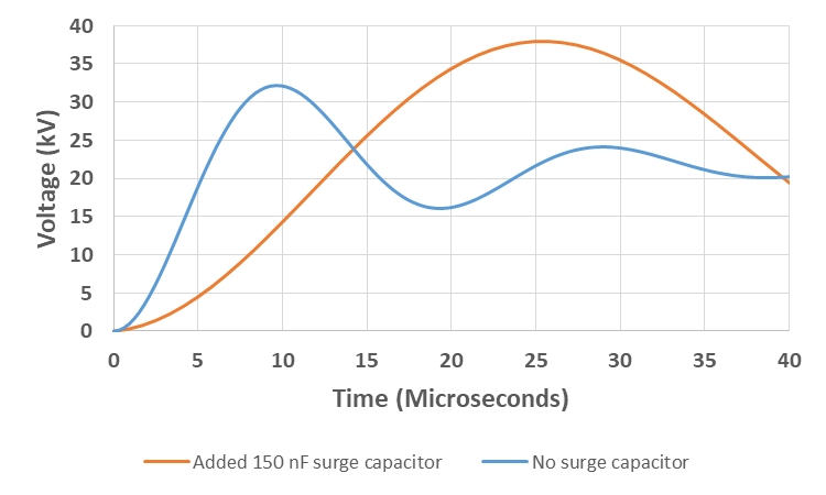
Figure 8 - System-source fault for 17.5 kV rated circuit breaker and 100 kA fault level without and with added surge capacitor at 150 nF
Surge capacitors are commonly applied on both sides of the circuit breaker and the effect of such a capacitor at 150 nF on the above example is calculated as follows. R and L are unchanged and only quantities involving C need to be re‑calculated, i.e. new values for dp and tg.
and
The equation for the TRV now is
and is also plotted in Fig. 8. In general the addition of surge capacitors will have the effect of shifting the curves in Fig. 2 upwards and to the right. In contrast, the alternative to reduce the RRRV using a circuit breaker opening resistor, will cause the curves to shift downwards in the direction towards overdamping.
The standard TRVs for the out-of-phase and load current switching cases with added surge capacitance have been the subject of some controversy and dedicated discussion.
The issues have been resolved by the addition of an Excel simulation-based tool with embedded calculations as part of the standard. This is the first time that a calculation of this nature is used in an IEC or IEEE standard. The required input is the generator voltage and MVA rating, system-source fault current rating, and the values of the surge capacitors. The tool output is the test uc and RRRV values for both the out-of-phase and load current switching cases. The use of the tool for the former case and the same circuit breaker as above is demonstrated in the following.
The input 17.5 kV, 190 MVA, 100 kA and 150 nF surge capacitors on both sides yields uc = 55.8 kA and RRRV = 1.9 kV/µs. Note that the standard generator-source fault current is taken at 50% of the system-source fault current rating and the out-of-phase angle is 90° giving a recovery voltage peak 30.31 kV with kpp = 1.5 pu.
This equation is plotted in Fig. 9 in comparison to the corresponding analytical calculation where the respective circuits are taken from the system-source and generator-source fault testing cases and the out-of-phase recovery voltage is split in ratio of the of the two circuit impedances. The latter calculation tends to yield a slightly faster RRRV and a lower peak value than the more comprehensive IEC tool calculation.
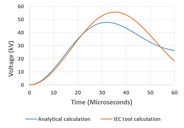
Figure 9 - Calculated TRVs using the analytical approach and the IEC tool for 17 kV, generator circuit breaker out-of-phase switching with added surge capacitors
4. Discussion and Conclusion
In spite of today’s prevalent use of simulation software, a knowledge of analytical calculation methods is essential for two reasons. Firstly, the methods provide an understanding and appreciation of the roles and influences of R, L and C alone or in combination in series and parallel circuits as they relate to TRV attributes. Secondly, the methods provide a means for comparison to determine if simulation study results are acceptable. In addition an estimation of TRVs in substations is possible using the guidance provided in the IEEE guide [5]. The key conclusion is that the generalized approach is applicable to all fault and load current switching cases and is readily usable to determine the effects of added surge capacitors and series reactors.
5. Appendix : General solutions for second order differential equations
Second order linear homogenous differential equations take the form
where a, b and c are constants. x(t) = ert is a solution for the equation and substitution yields
where the term within the bracket is the so-called characteristic equation which equals zero (ert ≠ 0) with roots r1 and r2 given by
The solution for the differential equation, it being second order, must have two arbitrary constants and is given by
A and B are determined from the boundary conditions, also referred to as initial conditions.
To simplify x(t), take
giving
and
x(t) can take three forms dependent on being real, zero or complex and the outcomes are shown in Table A1 where k1 and k2 are constants derived from the above-noted boundary conditions.
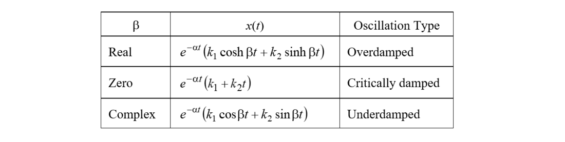
Table II - x(t) Solutions
A second possibility is that the second order differential equation is non-linear and inhomogeneous of the form
This type of equation is solved in part as discussed above and in addition using the method of undetermined coefficients.
References
- A. Greenwood and T. H. Lee, “Generalized damping curves and their use in solving power-switching transients,” AIEE Transactions 85, August 1963.
- A. Greenwood, “Electrical Transients in Power Systems,” John Wiley & Sons Ltd., 1971.
- C. H. W. Lackey, “Some technical considerations relating to the design, performance and application of high-voltage switchgear,” Transactions South African Institute of Electrical Engineers, September 1951.
- D. F. Peelo, “Current Interruption Transients Calculation,” Wiley IEEE Press, February 2020.
- C37.011-2019—IEEE guide for the application of transient recovery voltage for AC high-voltage circuit breakers with rated maximum voltage above 1000 V.
- IEC 62271-306—Guide to IEC 62271-100, IEC 62271-1 and other IEC standards related to alternating current circuit-breakers.
- IEC/IEEE 62271-37-013—Alternating current generator circuit breakers.
Biography
David Peelo is a graduate of University College Dublin and the Eindhoven University of Technology, a former switching specialist at BC Hydro and is now an independent consultant. He is an IEEE Distinguished Lecturer, a Distinguished Member of CIGRE and chairs the Canadian National Committee for IEC Technical Committee 17 and Subcommittees 17A and 17C. He is the author of a textbook on transient recovery voltage calculation and has co-authored two other textbooks on switchgear and switching including a CIGRE Green Book.