Ground modeling for the design of electrical grounding systems - The determination of the geoelectric model depth
Author
P.E. DA FONSECA FREIRE - Consultant Paiol Engenharia, Paulínia/SP, Brazil

Summary
The problem here proposed is the determination of the required depth of the geoelectric model to be used in the design of the grounding system of wide-area renewable power plants, kilometers sized, which shall be compatible with the plant area and the tectonic setting of the site. Sites located within low resistivity sedimentary basins require shallower geoelectric models, while those located within high resistivity cratonic areas require deeper geoelectric models. Based on the knowledge of the tectonic setting of the site, the geoelectric model depth can be estimated and the ground surveys can be specified, which may include a combination of shallow vertical electrical soundings (VES) with audiomagnetotelluric (AMT) and/or time-domain electromagnetic (TDEM) surveys. In this paper, a parametric study evaluates the required geoelectric model depth for a windfarm and two sizes of photovoltaic power plants. This multidisciplinary paper applies geophysics knowledge to the solution of an engineering problem.
Keywords
geoelectric modeling - ground resistivity - grounding - photovoltaic power plants - windfarms1. Introduction
40 years ago, when I was just graduated in electrical engineering, a big grounding grid was a substation yard with up to 20.000 m². Nowadays wide-area grounding systems have dimensions of kilometers, usually associated with windfarms and solar plants. However, for most of the projects, these wide-area grounding systems are still designed similarly as it is done for power substations, using shallow geoelectric models obtained from vertical electrical surveys, using low-power AC resistivity meters, with the Wenner arrangement and current probes spacing limited to 100 m.
In this paper, three layers’ 1D geoelectric models are suggested for three basic tectonic settings, considering three eons – “Archean” (> 2.5 Ba), “Proterozoic” (> 541 Ma), and “Phanerozoic” (< 541 Ma). These basic geoelectric models are used for the development of a parametric study to evaluate the sensitivity of the grounding resistance to geoelectric models that represent different tectonic settings. Three grounding systems of different patterns and dimensions were studied - a windfarm, which has a linear topology with concentrated groundings distributed along an interconnecting medium-voltage power line, and two sizes of solar plants, with matrix pattern grounding grids.
The definition of the depth of the geoelectric model is important because a model that is not deep enough will result in wrong ground potential rise (GPR) calculations, and thus in bad estimates of the electrical performance of the grounding system. However, a too deep model may imply unnecessary ground surveys and introduces complexity and processing time to the grounding system simulation.
This same methodology has already been applied to the evaluation of the geoelectric model depth for the ground electrodes of High Voltage Direct Current (HVDC) transmission systems [1].
The parametric study was performed with the MALZ module of CDEGS software [2], considering three-layer 1D geoelectric models that reproduce three different tectonic settings. The 1D geoelectric model can be associated with a sedimentary basin, with horizontal and parallel-ground layers. Despite its limitations for the application to wide areas, which in most cases probably show a 3D structure, the 1D geoelectric model is the traditional model used in the electrical grounding industry and is available for most of the software for the simulation of grounding systems.
It was calculated the grounding resistance of an aerogenerator tower, of a windfarm with two options of grounding system and two solar plants with different sizes, as a function of the depth of the top of the basement, which is the high-resistivity bottom layer of the geoelectric model. The simulations were performed for increasing widths of the intermediate ground layer, resulting in the deepening of the basement, to search for the depth at which the grounding resistance of the simulated system would not be affected within a misfit established as 5%.
The control parameter selected for this analysis is the grounding resistance. Another important parameter of the grounding system’s electrical performance is the soil surface potential profile, which can be expressed by a potential x distance curve, for the 1D ground structure. This curve defines the step and touch potentials given the injected current into the grounding system. The deeper ground layer is not expected to interfere significantly with the potential gradients that will occur close to the grounding elements.
2. The depth of penetration of electrical currents into the earth’s crust
Carson [3] proposed a method of calculating the AC transmission line frequency-dependent impedance considering the contribution of the ground return. Carson’s method expresses the impedance by employing an improper integral that shall be expanded into an infinite series for computation. These integrals can be approximated using proper numerical integration methods [4]. Carson’s formulation considers a homogeneous ground with relative permeability unitary; neglects the displacement currents in the air and the ground, and considers the field propagation quasi-TEM (Transverse ElectroMagnetic).
Deri et al. [5] suggested that the ground can be replaced by an ideal plane, placed below the soil surface at the complex penetration depth of a plane wave with the system frequency (Figure 1). The main advantage of this model is that it allows for the use of simple formulae for the calculation of self and mutual impedances of the conductors of transmission lines, derived from its complex images, producing results that match those obtained from Carson’s correction terms, which are much more complicated to calculate. The complex depth of earth return method assumes that the current in the overhead conductor returns through an imaginary section of ground located directly under the line and replaces the ground section with an equivalent return conductor.
Considering Figure 1.3, the complex depth of the equivalent return conductor will be (in meters).
Sunde [6] proposed the equation for the calculation of the ground impedance of a single-wire overhead line, which introduces the complex ground propagation constant:
, where;
- w = 2πf – angular frequency (Radians/s),
- μ0 – magnetic permeability of the free-space (4π 10-7 H/m),
0 – dielectric constant or permittivity of the free-space = 1/(μ0 c2) = 8.854 10−12 F/m,
The parameter γ can be associated with the diffusive penetration of a plane electromagnetic wave into the ground. Considering the low frequencies of the AC transmission systems, it is possible to disregard the second term of , related to the displacement currents, reducing the propagation constant to
, which is the inverse of
, the complex depth of the image plane:
Neglecting h, applying tothe relations of square root and reciprocal of complex numbers, and working with the modulus of
, it is possible to define the penetration depth:
(in meters)
This result means that the penetration into the ground of the return current is a diffusive process, with attenuation ruled by an exponential decay, which for frequencies below 1 MHz can be expressed as a function of the current density at the soil surface (Js) by:
.
In practice, the analysis is more complex, because the subsurface geoelectric structure is never uniform, presenting layers and volumes of different resistivity, depending on the terrain traversed by the transmission line. An AC three-phase transmission line with a phase-to-ground short-circuit at one of its ends, has the phase circuit closed by ground return, with the current flowing back along the path of the line, from the short-circuited end to the transformer grounding at the feeder end. This return current, having the entire semi-volume of ground to circulate, seeks the path of least impedance, following the path of the line because of the magnetic coupling between the current in the line’s phase conductor and the return current in the ground. (Figure 2).
The ground section traversed by the return current can be determined by the penetration depth (), which characterizes the “skin effect” that is the depth (in meters) at which the current density per unit of the ground section is reduced to 1/e (1/2.718 ~ 37%) of its value at the soil surface (Figure 3). The exponential decay of the current density occurs also laterally, limiting the width of the ground current row below the transmission line. The ground current density can be considered negligible at a distance higher than 3d on each side of the row axis.
A long transmission line operating at 60 Hz above a 400 Ωm homogeneous ground resistivity, has a penetration depth () of 1300 m. The current lines in the ground will run parallel along the path of the transmission line, except at its ends, where they converge/diverge towards the grounding electrodes. At each end of the line, a “terminal effect" occurs within a ground volume of about 3
radii, adding a component to the impedance of the path, which is defined as the grounding grid resistance. As the frequency increases, the inductive reactance becomes more dominant in this process, driving the current to minimize the magnetic flux linkage with the physical line, following the same path closer to the line, through a ground section each time smaller, which can be interpreted as the "skin" effect, the circulation in a section of ground increasingly shallower and narrower. If by hypothesis the line operates at a frequency of 25 kHz, then
will be reduced to about 5% of the above-calculated value, i.e. 64 m.
Contrarily, if the frequency is successively reduced, the return current will increasingly spread into the ground, and the equivalent return path will become increasingly deeper and wider. When the zero frequency is reached, which is the case of the HVDC line, the scattering is complete, and the return path will be down to an infinite depth. At this point it can be said that the ground electrodes are decoupled at both ends of the HVDC line, meaning that the impedance of the path disappears, leaving only the terminal effect, which becomes the resistance of the grounding electrodes.
The conclusion is that DC currents penetrate deep into the Earth’s crust, however, AC currents penetrate only down to the so-called, near-surface depths, no more than a few kilometers depth for the higher resistivity grounds.
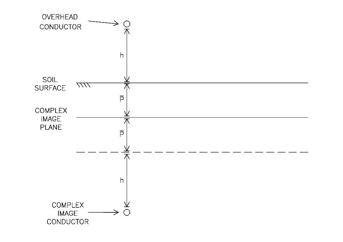
Figure 1 - geometry of an overhead conductor with ground return, with the illustration of the complex plane of symmetry and the complex penetration depth
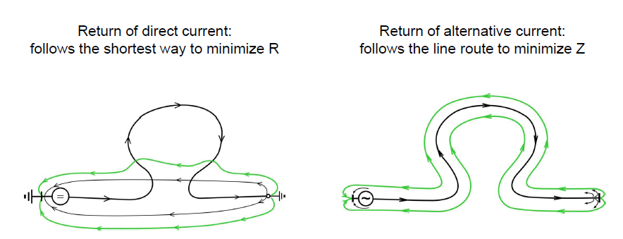
Figure 2 - ground return for an AC line – the current follows the path of the line
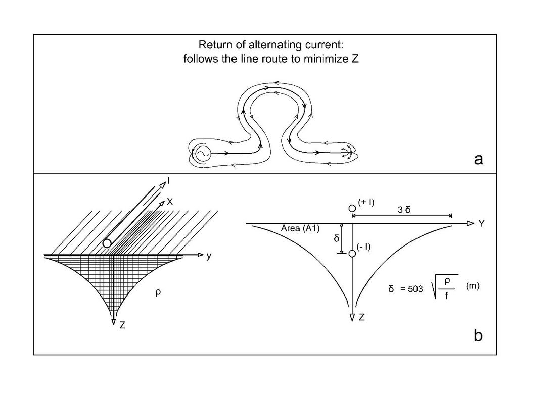
Figure 3 - ground sections associated with the ground return of DC and AC currents, [modified from 3]
3. Earth’s crust structure
The cratons (from the Greek cratos, meaning strength) occupy most of Earth's continental lithosphere, being the large and stable crustal blocks that have attained stability and have been little deformed, remaining coherent and relatively rigid since the Precambrian Supereon (> 541 Ma ago). The cratons are the stable nuclei of the continents, being eroded remnants from ancient continents, cold and thick segments of the lithosphere, to which younger parts of the crust have been added, surviving several tectonic processes. The cratons occupy the largest area of the continental crust (70%), with an average thickness of about 35 km, and can be divided into the following units:
- Archaean cratonic nuclei (> 2500 Ma old) - crystalline basement undeformed in the Phanerozoic Eon (last 541 Ma), constituting only 7% of the total area of the continental crust;
- shields - upraised rocks of the Precambrian (older than 541 Ma) crystalline basement, which constitute 30% of the exposed surface of the continents;
- platforms - eroded shields of Precambrian rocks, consolidated during earlier deformations, overlain by sub-horizontal and younger layers of sediments.
The continental crust is extremely heterogeneous in the three dimensions and is divided into geologic provinces, which are large spatial units characterized by similar geologic history and evolution. The continents are built from the combination of very old cratonic nucleus, sutured at the mobile belts (along the collision lines), forming the shields, which are the exposed and stable cratonic crust areas, surrounded by the platforms, where the cratonic crust is overlain by a flat-lying sedimentary cover. The continental shelf is the submerged area bordering the continents, flat but with a slight seaward slope from the shoreline to a depth of 200 m, where the continental slope begins. The primary geological provinces include other structures, such as orogens – subjected to recent or ancient mountain building; continental basins – subsided areas covered by sedimentary accumulations of variable thickness; large igneous provinces - covered by extensive igneous extrusions, usually 1–5 km thick; rifts and extended crust – where horizontal extension resulted in the subsidence/thinning of the crust [7].
4. Continental upper crust geoelectric models
The simplest model for the representation of Earth’s crust geoelectric structure, as viewed from a point on the soil surface, is the horizontally layered 1D model (orthotropic model). Jones [8] suggests three 1D geoelectric models for the generic continental crust, according to its age - “Archean” (> 2.5 Ba), “Proterozoic” (> 541 Ma), and “Phanerozoic” (< 541 Ma). The upper crust for the Archean model is expected to be very resistive (up to 40000 Ωm), the Proterozoic model presents high resistivity (up to 10000 Ωm), and the Phanerozoic model of moderate resistivity (up to 1000 Ωm).
The superficial ground layers, where the rocky basement is not outcropping, are usually formed by porous sedimentary rocks, of varying depth, with connected pores and sometimes saturated with saline fluids. Compaction and cementation, however, reduce pore space and connectivity, thus increasing resistivity with depth. In the case of cratonic areas, beneath the sedimentary cover, the upper crustal rocks are generally very resistive; however, in sedimentary basins, the resistivity of the basement is not so high, due to the fractured and water-saturated rocks, faulted and altered by tectonic processes, and metamorphosed by the water and pressure above it.
Vozoff [9] suggests the typical magnetotelluric response for a sedimentary basin, characterized by the apparent resistivity curve and corresponding 1D geoelectric model of Figure 4, which reveals the basic 3-layered 1D model, from the soil surface down to the rocky basement.
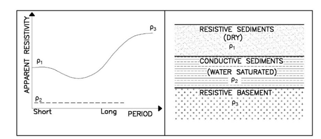
Figure 4 - typical MT response and geoelectric model for a sedimentary basin [modified from 4]
Basic 3-layers 1D geoelectric model:
- superficial and dry ground - medium to high resistivity
- phreatic or aquifer - water-saturated sediments with low to medium resistivity
- basement - medium to high resistivity
5. The adopted three-layer geoelectric model
Vozoff’s three-layer geoelectric model was adopted for the development of the parametric study, considering a shallow layer, with a few tens of meters width, and a near-surface layer, above the rocky basement from 100 m to two-kilometer depth. For this study, based on this triple-layer structure, it was established three geoelectric models, corresponding to high, medium, and low resistivity environments (Figure 5).
The shallow ground layer was defined with a maximum depth of 50 m, with resistivities of 250 Ωm, 1000 Ωm, and 10.000 Ωm. The intermediate ground layer was defined with a maximum depth of 2000 m, with resistivities of 100 Ωm, 500 Ωm, and 1.000 Ωm, requiring for its survey an electromagnetic sounding method (AMT and/or TDEM). These two ground layers were combined with three basement resistivity options - 1000 Ωm (Phanerozoic), 10.000 Ωm (Proterozoic), and 40.000 Ωm (Archean), as proposed by Jones [8]. Figure 2 illustrates the three geoelectric models. For the parametric study, the width of the intermediate ground layer varied from 100 m to 2000 m, allowing for the simulation of a wide range of geoelectric structures.
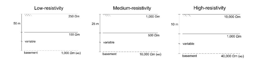
Figure 5 - the three geoelectric models adopted
6. Simulated windfarm and solar plant configurations
For the development of this study, it was established a typical configuration of a windfarm, which has a linear pattern. The solar plant has a matrix pattern and because this kind of generating plant can have a wide area variation, it was selected two configurations for the parametric study.
6.1. The windfarm configuration
The windfarm has 19 wind generators, rated 3 MW, aligned along 5.2 km, which means an average tower’s spacing of 290 m. They are interconnected by a 34.5 kV double-circuit aerial line, which converges into a high-voltage substation (Figure 6). The substation grounding grid has an average mesh size of 10 m. The grounding of each tower includes the steel reinforcements of the tower’s foundation, connected to three bare copper rings around the tower base plus two 50 m radial 50 mm² copper conductors [10]. The 34.5 kV lines shield-wires allow for the interconnection of the tower’s groundings, and two options for this interconnection were studied in this paper – through an aerial shield-wire or by a bare cable buried along with the entire extension of the medium-voltage line, in both cases using a 7x8 AWG copper-steel conductor (Ø 9.78 mm with 58.6 mm²).
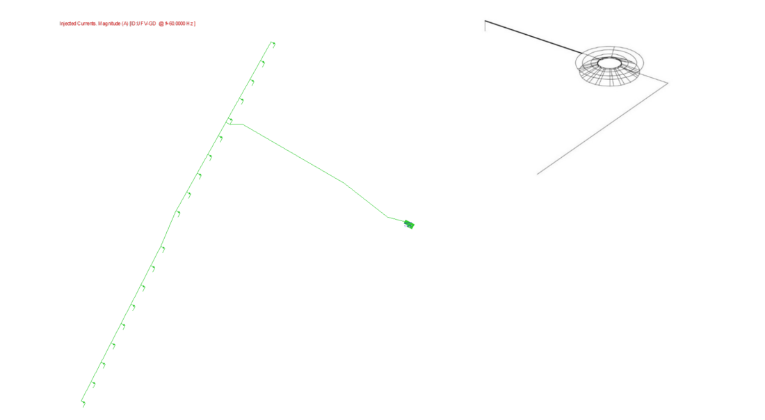
Figure 6 - windfarm configuration – 19 towers along 5.2 km (average spacing of 290 m), with detail of the grounding configuration of one tower (including the foundation reinforcement steel)
6.2. The solar plant configurations
Solar photovoltaic generating plants present a wide range of configurations and modes of installation, which can be rooftop, floating, and ground facilities. It was considered here two dimensions of ground photovoltaic plants – the smaller with 5 MWp and a big one with 500 MWp, as illustrated in Figure 7.
The smaller solar plant is divided into 5 sectors, each sector connected to a skid where the DC energy is converted to AC and stepped up to 34,5 kV. The five step-up transformers are paralleled in a medium-voltage substation, which interfaces the connection of the photovoltaic plant with the distribution line of the power utility. The grounding system model for this solar plant includes 1.000 steel stakes stuck 2 m into the ground, which support the photovoltaic panels, interconnected by 3.000 m of 50 mm² bare copper conductors.
The bigger solar plant is divided into 62 sectors, each sector connected to a conversion unit, which is a skid where the DC energy is converted to AC and stepped up to 34,5 kV. The 62 conversion units are connected to a high-voltage substation where the energy is stepped up to 500 kV and injected into the interconnected national power system.
The grounding grid model for this solar plant was simulated by 150 km of 50 mm² bare copper conductors, which interconnect the trackers of the 62 sectors of the plant. As a conservative approach, the thousands of steel stakes stuck into the ground for supporting the photovoltaic panels were not considered.
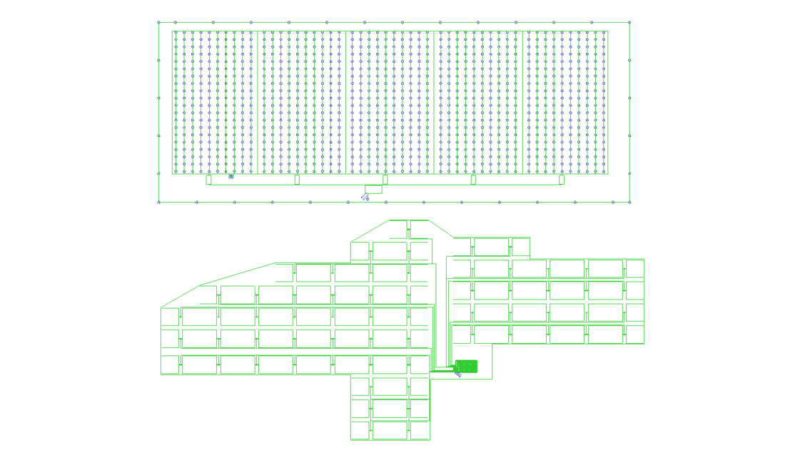
Figure 7 - grounding system configuration for the 5 MWp solar plant (620 m x 240 m, ≈150.000 m²) and the 500 MWp solar plant (5,7 km x 2,5 km, ≈7.9 km²)
7. Results of the simulations
7.1. Windfarm Simulations
The first simulations evaluated the grounding performance of a single aerogenerator tower, as illustrated in Figure 6. The complete windfarm, with its 19 aerogenerator towers was simulated for two interconnection conditions – through the 34,5 kV transmission line shield wire or by a buried grounding conductor, both using a 7x8 AWG copper-steel conductor. The typical aerogenerator specification requires a tower grounding resistance below 10 Ω. Until 2019 the IEC 61400-24 standard [11] also recommended the maximum 10 Ω resistance, however, the 2019 review eliminated this recommendation.
7.1.1. Simulation of a Single Tower Grounding
Table 1 shows that the effect of a higher resistivity ground layer below 50 m depth does not have a significant effect on the performance of the isolated tower grounding. Therefore, a shallow ground resistivity survey will be enough for the modeling of the grounding of a single aerogenerator tower.
However, the simulations show that for medium and high-resistivity shallow grounds it shall be expected tower grounding resistances that are higher than the required 10 Ω. This is a frequent situation because in many projects the aerogenerator towers are located on the top of rocky hills, where the ground resistivities are higher. In this case, the complete windfarm shall be simulated, to verify if the interconnection of the towers’ groundings will allow for the achievement of the required 10 Ω grounding resistance.
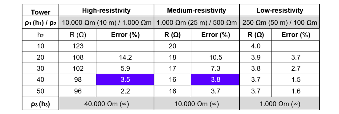
Table 1 - calculated grounding resistance of an aerogenerator tower (blue marked for the resistance deviation < 5%)
8. Simulation of the grounding system of the complete windfarm
Tables 2 and 3 show that the simulation of the grounding system of the complete windfarm allows for achieving the required 10 Ω resistance, as viewed from a tower located in the middle of the windfarm. However, the proper calculation of this parameter requires a geoelectric model depth of a few hundred meters. Therefore, the shallow ground resistivity survey developed at the towers’ location shall be combined with an electromagnetic sounding survey developed along the previewed windfarm path, for the acquisition of data for the construction of a half-kilometer depth geoelectric model, which will allow for a resistance calculation with an error below 3%.
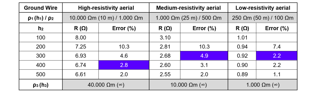
Table 2 - calculated resistance of the windfarm grounding system with interconnections by an aerial 7x8 AWG copper-steel shield wire (blue marked for the resistance deviation < 5%)
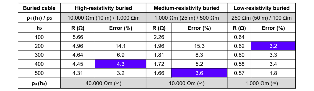
Table 3 - calculated resistance of the windfarm grounding system with interconnections by a buried 7x8 AWG copper-steel conductor (blue marked for the resistance deviation < 5%)
8.1. Solar Plant Simulations
Tables 4 and 5 show the calculated grounding resistances of the two solar plants, as viewed from the collecting substation. It was found that the 5 MW plant requires a one-kilometer depth geoelectric model and the 500 Mw plant requires a two-kilometers depth geoelectric model.
Therefore, the design of the grounding system of a ground solar plant requires that the shallow ground resistivity survey developed within the plant area shall be complemented by an electromagnetic sounding survey. The data acquired by the two surveys shall be combined for the construction of a one or two-kilometer depth geoelectric model, depending on the plant size and tectonic setting. It is interesting to note that the one-kilometer depth geoelectric model has a dimension that is wider than the 5 MW solar plant diagonal (typically about 600 m).
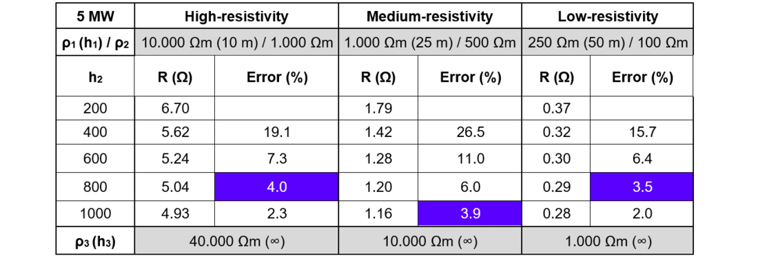
Table 4 - calculated grounding resistance of the 5 MW solar plant (blue marked for the resistance deviation < 5%)
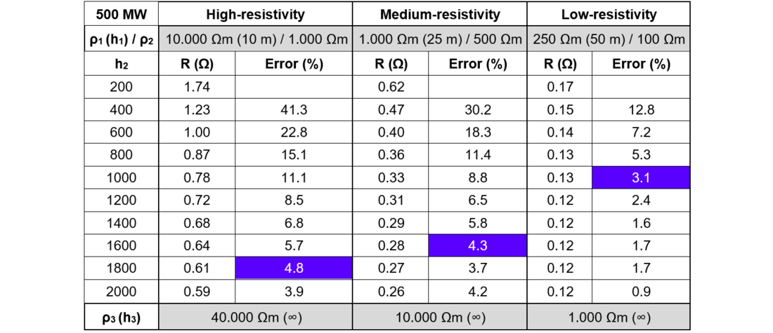
Table 5 - calculated grounding resistance of the 500 MW solar plant (blue marked for the resistance deviation < 5%)
9. Conclusions
The first finding of this set of simulations is that if the complete grounding system is considered, there is no reason for worries concerning the final resistance of windfarms or solar plants because these wide-area power plants will always present a low grounding resistance, below the 10 Ω reference.
For the design of HVDC ground electrodes, it is required a deep geoelectric model, which may reach the entire upper crust (about 20 km depth) [1]. For an AC wide-area grounding system, a 2 km depth geoelectric model will be enough, even within a high-resistivity environment.
For a single aerogenerator tower of a windfarm, the traditional electroresistivity survey with a Wenner arrangement and spacing up to 64 m will be enough for the construction of a good geoelectric model. However, for the wide-area generating plants here analyzed, the construction of a geoelectric model requires the combination of shallow vertical electrical soundings (VES) with near-surface electromagnetic data, such as audio-magnetotelluric (AMT) and/or time-domain electromagnetic (TDEM) soundings.
The Brazilian standard for ground resistivity surveys and geoelectric modeling was reviewed in 2020 [12] and now includes the electromagnetic surveys, considering its application for wide-area grounding systems. The methodology for the construction of a deep geoelectric model, combining electrical and electromagnetic data, was initially established for the design of HVDC ground electrodes [13, 14]. This methodology has already been applied for the geoelectric modeling of four wide-area renewable power plants, two windfarms [15] and two solar plants (with 475 MWp and 766 MWp).
The parametric study here presented adopted a 3-layers 1D geoelectric model. However, for a wide-area grounding system design, more ground layers are required, to allow for a good representation of the average shallow ground layers, which are responsible for the soil surface potential gradients. It is beyond the scope of this work the presentation the methodology for the construction of the complete geoelectric model, from the soil surface down to the required depth.
References
- P. E. F. Freire, S. Y. Pereira, “HVDC Grounding Electrodes and Tectonic Setting”, B4-102, Cigre Session 2018.
- CDEGS and MultiFields Software Packages, Safe Engineering Services & technologies ltd., Montreal, Quebec, Canada, 2009.
- J. R. Carson, “Wave propagation on overhead wires with ground return”, Bell Systems techn., Vol. 5, pp. 539-554, 1926.
- G. Varju, “Earth Return - phenomena and impedance”, Budapest University of Technology & Economics, PowerPoint Presentation.
- A. Deri, G. Tevan, A. Semlyen, A. Castanheira, “The complex ground return plane, a simplified model for homogeneous and multilayer earth return”, IEEE Transactions on Power Apparatus and Systems, Vol. PAS-100, pp. 3686-3693, Aug. 1981.
- D. Sunde, “Earth Conduction Effects in Transmission Systems”, Dover Publications, New York, USA, 1948.
- CMR. Fowler, “The Solid Earth – An Introduction to Global Geophysics”, Cambridge University Press, 1990.
- A. G. Jones, “Imaging and Observing the Electrical Moho’, Tectonophysics 609, pp. 423–436, 2013.
- K. Vozoff, “The Magnetotelluric Method in the Exploration of Sedimentary Basins”, Geophysics 37(1): pp. 98-141, 1972.
- P. E. F. Freire, S. P. Yoshinaga, “Windfarm Grounding”, 2016 CIGRE C4 International Colloquium on EMC, Lightning, and Power Quality Considerations for Renewable Energy Systems.
- IEC 61400-24, “Wind turbine generator systems –Part 24: Lightning protection”.
- P. E. F. Freire, J. H. Zancanela, H. Takayanagi, J. A. Jardini, “The Review of The Brazilian Standard NBR-7117 - Ground Resistivity Surveys and Geoelectric Modeling. International Conference on Grounding & Lightning Physics and Effects”, Belo Horizonte, Brazil, June 2021.
- P. E. F. Freire, S. P. Yoshinaga, A. L. Padilha, “Adjustment of a Crustal Geoelectric Model from Commissioning Data of HVDC Ground Electrodes: A Case Study from the Northeastern Paraná Basin, Brazil”, Journal of Applied Geophysics 182 (2020) 104186, DOI: 10.1016/j.jappgeo.2020.104186.
- P. E. F. Freire, S. P. Yoshinaga, A. L. Padilha, “Adjustment of the Geoelectric Model for a Ground Electrode Design – the case of the Rio Madeira HVDC Transmission System, Brazil”, Cigre Science & Engineering, Feb. 2021.
- P. E. F. Freire, C. Schweig, B. Kriegshäuser, P. de Lugão, JL. Porsani, N. R. A. Silva, J. Z. Minatto, “Geoelectric Modeling for the Retrofit of the Grounding System of the Bom Jardim da Serra Windfarm”, Brazil Windpower 2020 - International Conference on Grounding & Lightning Physics and Effects, Belo Horizonte, Brazil, June 2021.
Biography
Paulo Edmundo da F. Freire was born in Rio de Janeiro, Brazil, in 1955. He graduated (1978) and received a master (1984) degrees in electrical engineering from the Pontificia Universidade Católica do Rio de Janeiro, and a Ph.D. degree in geosciences, from UNICAMP – University of Campinas, São Paulo (2018).
Since 1990 he runs his own consulting company (PAIOL Engenharia), and his special fields of interest are grounding and lightning protection systems. He is a member of CIGRE and an active member of the standardization committee in Brazil. He has presented/published about 45 papers in technical seminars/journals in Brazil and abroad.