Harmonic Emission Assessment of Solar Farms: a Comparative Study Using EMT and Frequency Domain Models
Authors
S. LIYANAGE, S. PERERA, D. ROBINSON
University of Wollongong, Australia

Summary
Large-scale solar farms connected to electricity networks have to demonstrate pre-connection harmonic compliance. To assist this, network service providers use vendor-provided Thevenin/Norton harmonic models of the associated inverters, which are based on off-site tests and modelling. It is questionable as to whether these frequency-domain models can replicate the true behaviour of geographically scattered inverters connected to the point of common coupling via underground cables. The primary objective of this paper is to examine possible discrepancies that can arise in the use of such models by comparing the corresponding outcomes with those established using time-domain models of the inverters. The broad conclusion is that Thevenin/Norton models are unable to reliably predict the true harmonic behaviour in actual operating environments. The study outcomes also support the arithmetic addition of the harmonic currents contributed by the individual inverters to the resultant harmonic current level at the solar farm grid connection point in the absence of resonance conditions.
1. Introduction
The number of large-scale solar photovoltaic (PV) generating plants connected to electricity grids is on the rise in many parts of the world [1]. This unprecedented growth of PV systems is intertwined with a range of technical challenges. Among these are the power quality problems of concern and in particular, the harmonic issues which arise as a result of power electronic interfaces (inverters) used [2].
Notably, the low-order harmonics up to 50th order are required to be managed to ensure that networks meet the planning levels adopted by the network operators. In order to satisfy this requirement, PV plants need to be provided with harmonic current/voltage emission allocation levels by network operators [3]. To evaluate the harmonic voltages that transpire at the point of common coupling (PCC) subsequent to the PV system connection, the network harmonic impedance profiles evaluated at the PCC for various network operating scenarios of relevance and the harmonic currents injected into these harmonic impedances are required. In comparison to the use of ideal current sources to represent the harmonic behaviour of each inverter within a PV plant, it is the current practice to use inverter vendor provided Norton/Thevenin harmonic models [4] of which the parameters are established through simulations and/or measurements under chosen conditions which include multiple power output levels at unity power factor. It is understood that the models provided for each harmonic order refers to the worst case noting that inverters can operate over a wide range of power output levels in practice and hence their variability based on power output levels is ignored in harmonic studies. With this it is also important to note that the harmonic magnitudes do not exhibit a linear relationship with the power output level of an inverter. Further, the influence of the network within a specific solar plant containing a collection of inverters, the underground cable system and the network external to the solar plant are not represented in the determination of such models carried out under chosen conditions. In addition, there is the possibility of interactions between the different inverters in a PV plant that can alter their harmonic emission behaviour, which are not represented when fixed Norton/Thevenin harmonic models of inverters are used for harmonic assessment of the plant. Despite this is seen to be the case, the fixed vendor provided Norton/Thevenin harmonic models are used together with the detailed models of the cable reticulation system and the connected power system in pre-compliance studies and the accuracy of the use of such models is questionable with regard to harmonic compliance studies.
The possible phase angle diversity that can exist between the individual harmonic currents of the different inverters in a solar plant is not taken care of in the use of Norton/Thevenin models, although one can argue the use of the well-known general summation law as used in IEC 61000.3.6 [5]. It is, however, important to note that the above general summation law is generally applied to installations that are usually independent of each other in their operation, whereas in a single solar plant, all inverters are usually controlled by the same power plant controller. It is also worth noting the work of [1], which refers to the case of identical inverters used to build up a solar farm, the total harmonic current at the PCC is suggested to be the arithmetic sum of the individual inverter harmonic currents. On the contrary, studies in [6], [7] have aimed to find an appropriate method to calculate the aggregated harmonic current at the PCC. On the whole, the existing approaches on harmonic summation still leave room for further investigations to reach outcomes that are true to life.
Considering the number of hypotheses raised above associated with the validity in the use of Norton/Thevenin models of inverters, the work presented in this paper compares the results derived using electromagnetic transient (EMT) models of inverters in a PV plant environment with those derived using Norton/Thevenin models of the identical inverters in the same PV plant environment.
One of the significant challenges in carrying out this study is the unavailability of vital details of practical MW-scale inverters used in practice, including the details associated with the control systems, power electronic inverter switching strategies and many other components. Despite this difficulty, the time domain models developed using EMT software presented in Section 2 employ generic but industry recognised control techniques, well-known switching strategies and component details, which are as realistic as possible to represent each inverter.
The establishment of Norton/Thevenin harmonic models at a selected number of characteristic harmonic frequencies (5th, 7th, 11th, 13th) for the inverter model developed in time domain is given in Section 3. The key details of the solar farm model are given in Section 4. Section 5 presents an analysis of the performance of the Thevenin equivalent model used together with the cable network. In concluding, Section 6 gives a discussion on the applicability of summation laws with regard to the establishment of aggregated harmonic current at the PCC. Concluding remarks are given in Section 7.
2. Three-phase inverter model
A grid-connected three-phase voltage source inverter was developed using EMT software so that a number of these models can be used to represent a large solar farm environment. Some of the key parameters of the inverter are given in Table 1.
| Parameter | Value |
|---|---|
Inverter rated power | 2.5 MW |
Inverter DC link voltage | 1 kV |
Inverter switching frequency | 3 kHz |
Inverter transformer | 0.4/11 kV; 2.5 MVA; X = 0.04 pu |
Grid voltage/frequency | 132 kV/50 Hz |
Grid connection point (PCC) fault level | 2200 MVA , X/R = 10 |
Grid interfacing transformer | 11/132 kV; 100 MVA; X = 0.1 pu |
The formation and rating of the PV array were determined such that the intended rated power of 2.5 MW is achieved at the inverter output. The power losses across the low-pass filter components and the non-ideal inverter switches were also considered. The reference solar irradiance and the temperatures were taken as 1000W/m2 and 25°C respectively, while the inverter was designed to inject its rated power of 2.5 MW at the inverter output when the solar irradiance and the temperature are 900W/m2 and 25°C respectively. The maximum power point tracker (MPPT) and the DC to DC boost converter ensure the operation of the PV array at the maximum power point under changing solar irradiance and temperature conditions. Although different algorithms have been implemented, the incremental conductance algorithm was incorporated for the MPPT considering its advantages over the other available algorithms [8]. An LC filter of the inverter was modelled with a cut-off frequency of 400 Hz [9].
The inverter controllers have been noted to have a significant impact on the purity of the current supplied to the grid by a grid-connected inverter. Therefore, to regulate the inverter output current, a proportional-integral (PI) current controller with voltage feed-forward was modelled in the synchronous reference frame. The inner loop current controller ensures that the d-axis and q-axis current components follow the reference levels with a fast response. An outer loop controller, which controls the DC link voltage of the three-phase inverter was designed to generate one of the reference current components used in the current controller. The power control of the inverter was achieved employing the instantaneous power theory [10], [11], [12].
Space Vector Pulse Width Modulation (SVPWM) [13], [14] was chosen as the modulation strategy of the inverter model developed as it is a technique that is widely used in large inverters to generate switching pulses. SVPWM is a well-documented technique and effectively reduces the total harmonic distortion at the inverter output and allows achieving higher amplitude modulation indices compared with the Sinusoidal Pulse Width Modulation (SPWM), thus allowing greater DC link voltage utilization. The block diagram of the grid-connected three-phase inverter system is shown in Figure 1.
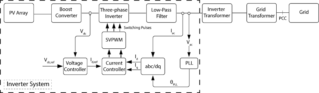
Figure 1 – Three-phase inverter system connected to the grid
Only the rated power operation at 2.5 MW was considered in this study. The corresponding harmonic spectrum of the output current as a percentage of the rated current is shown in Figure 2, where the total harmonic distortion (THD%) can be observed to be 0.786%.
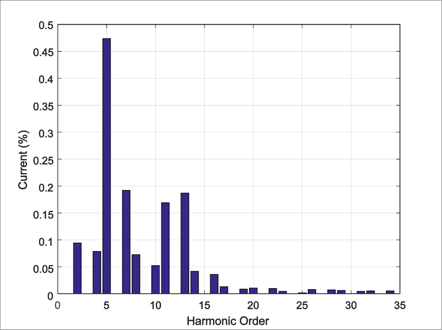
Figure 2 – Current harmonics at the PCC at the inverter rated power
3. Derivation of the inverter thevenin/norton equivalent harmonic models
It is traditional to use numerical and small-signal analysis methods in harmonic model development of non-linear systems such as inverters. For this reason, it was required to undertake such model development employing harmonic linearization techniques, which is a widely known technique that is used to develop small-signal linear models of time-varying systems [15]. This is done by superimposing a small harmonic signal on the output side of the inverter, which is followed by extraction of the required voltage or current components at the superimposed frequency to calculate the Thevenin or Norton model parameters [16], [17]. Since the order of significant harmonic components injected by a three-phase inverter are characterised by 6n±1, only 5th, 7th, 11th and 13th harmonics were considered in addition to the 29th and 31st harmonics while paying attention to their sequence properties. The total voltage on the grid side can be defined as given in (1) and (2) considering both positive and negative sequence harmonics stated above.
For positive sequence harmonic injection, the total input voltage can be written as,
(1)
where, V1, f1, Vp, fp and θp are fundamental voltage magnitude, fundamental frequency, positive sequence harmonic voltage magnitude, its frequency and phase angle respectively.
For negative sequence harmonic injection, the input voltage can be written as,
(2)
where, Vn, fn and θn are negative sequence harmonic voltage magnitude, its frequency and phase angle respectively.
The inverter output current that arises as a result of the externally applied resultant voltage can contain harmonics at different frequencies other than what is injected due to the non-linearity and operation of the inverters. Therefore, it is mandatory to remove all other harmonic components except the current and voltage components at the injected harmonic order to derive the intended small-signal source voltage and impedance of the inverter.
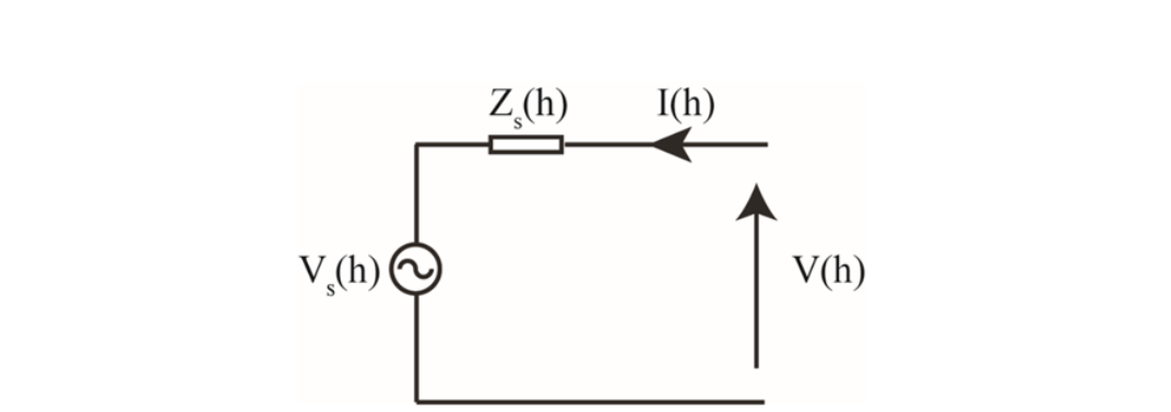
Figure 3 - Thevenin equivalent model of inverter representing its harmonic behaviour
If the inverter harmonic behaviour is represented using its Thevenin equivalent as shown in Figure 3, its parameters at the harmonic order (h) of interest can be derived using two independent current and voltage measurements taken at the inverter output in the frequency domain (using FFT analysis), and by applying equation (3) [18], [19], [20],
(3)
where, V1(h) and V2(h) are the two discrete voltage harmonic components measured at the inverter output terminals for the two discrete harmonic injection levels applied from the grid side. I1(h) and I2(h) are the current harmonics at the considered frequency, flowing into the inverter corresponding to those harmonic injection levels, respectively. Hence it is important to note that, the voltage (V(h)) that appears at the inverter output terminals is a result of the contribution of both the inverter and the background voltage and impedance.
The frequency-dependent Thevenin impedances Zs(h) and the corresponding source voltage Vs(h) can be derived using the expressions (4), where it is valid for any two different background conditions assuming the inverter operation is fixed.
(4)
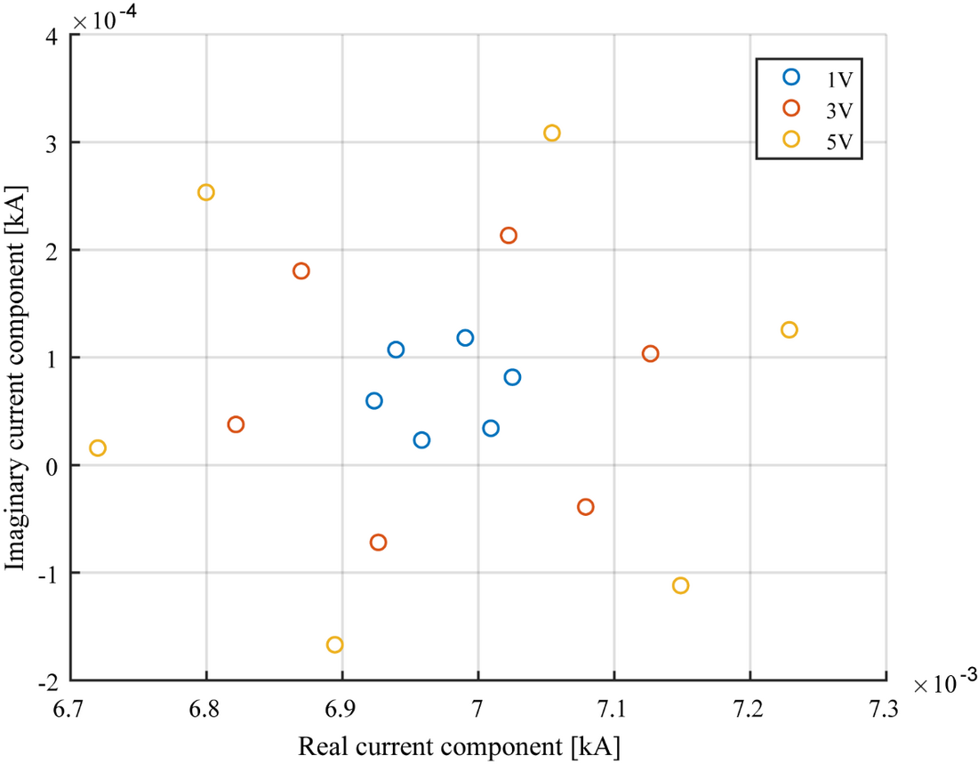
Figure 4 - Variation of the 7th harmonic current at the inverter terminal for different perturbation voltages
Voltages with three different magnitudes (1V, 3V and 5V), each of with six different phase angles (0°, 60°, 120°, 180°, 240° and 300°) were used as the harmonic voltages injected to the inverter system to investigate how the Thevenin equivalent parameters derived using (4) will vary depending on the magnitude and phase angle variations in the applied harmonic component. Figure 4 shows the current (I(f)) variation at the inverter output and Figure 5 shows the variation of Thevenin equivalent impedance and source voltage for the different harmonic voltages applied to the system for the 7th harmonic. From Figure 5, it is evident that the inverter Thevenin equivalent circuit parameters remain independent of the applied harmonic voltage magnitude or its phase angle.
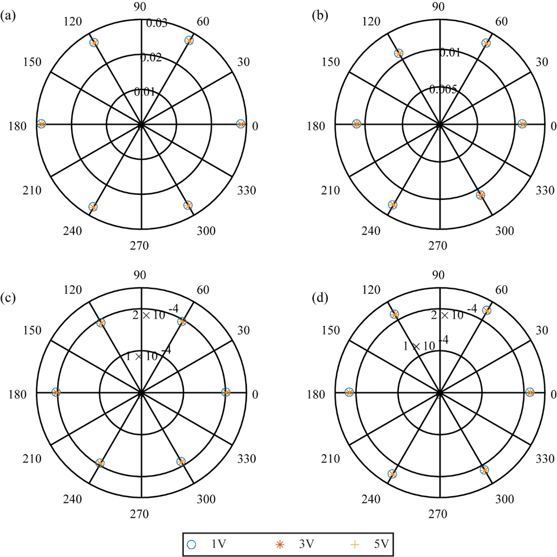
Figure 5 – 7th harmonic Thevenin equivalent impedance and source voltage variation (a) impedance - real part (b) impedance - imaginary part (c) voltage - real part (d) voltage - imaginary part
Thevenin equivalent circuit parameters derived following the process above for the harmonics under consideration are listed in Table 2.
| Harmonic Order | Thevenin Equivalent Impedance (Ω) | Thevenin Equivalent Source Voltage (kV) |
|---|---|---|
5 | 0.012 + j0.007 | 4.357E-04 ∠ -79.9° |
7 | 0.028 + j0.012 | 2.932E-04 ∠ 131.9° |
11 | 0.011 - j0.046 | 1.207E-04 ∠ -128.4° |
13 | 0.002 - j0.027 | 0.6775E-04 ∠ -96.7° |
29 | 2.350E-04 - j0.008 | 0.1255E-04 ∠ 122.2° |
31 | 2.243E-04 - j0.008 | 0.1115E-04 ∠ -50.0° |
To validate the derived Thevenin equivalent models, the EMT model of the inverter system (in Figure 1) was replaced with the Thevenin equivalent and the harmonic current at the PCC was extracted for each harmonic order. The results are compared with the current harmonic components measured at the PCC with the EMT modelled inverter connected to the grid. Resultant harmonic magnitudes for both cases are shown in Table 3. From these results, it can be concluded that a single inverter can be confidently replaced by its derived Thevenin model under the assumed conditions.
| Harmonic Order | With the EMT inverter model (kA) | With Thevenin Equivalent (kA) |
|---|---|---|
5 | 5.361E-05 | 5.353E-05 |
7 | 2.115E-05 | 2.113E-05 |
11 | 1.862E-05 | 1.884E-05 |
13 | 2.130E-05 | 2.157E-05 |
29 | 5.265E-07 | 5.209E-07 |
31 | 4.239E-07 | 4.266E-07 |
4. Solar farm model
In this study, a 12.5 MW solar farm with five identical 2.5 MW inverters was considered to maintain simplicity, although these five inverters are not sufficient to represent an actual large-scale solar farm. However, this small-scale farm was considered to be adequate to investigate the operational behaviour from a harmonic perspective.
A suitable underground cable network was included in the farm, which is an important part of any solar farm. This is often neglected in simplistic studies. However, it can significantly impact the harmonic behaviour at the PCC.
4.1 Cable network
The network harmonic impedance is highly dependent on the cable network. Cable length and the other parameters have been identified as influencing factors of the harmonic impedance associated with a solar farm. Moreover, compared with overhead lines, cables are more likely to exhibit resonance at lower frequencies due to the interaction between their capacitive reactance and the inductive reactance of the main transformer and the supply system [21], [22], [23]. Thus, accurate cable modelling is essential. Based on a real solar farm, realistic cable lengths, types and other parameters were incorporated in the study.
Considering the relatively short lengths of the cables in the considered solar farm, ∏ sections were used to represent the cable network in the simulation. The number of ∏ sections that need to be utilized (or the maximum frequency range represented by a ∏ model) can be calculated using (5).
(5)
where, F,N,v and l are the maximum frequency range, number of ∏ sections, propagation speed in km/s and line length in km respectively. From (5), it was confirmed that to represent each cable segment, a single ∏ section to be adequate. The solar farm layout is shown in Figure 6 where each inverter is connected to a 0.4 / 11 kV step-up transformer and connected via underground cables with different lengths to an 11 kV busbar. The 11 kV busbar is connected to the 11 / 132 kV grid transformer via a 2 km long cable. Parameters of the cables extracted using [24] are listed in Table 4.
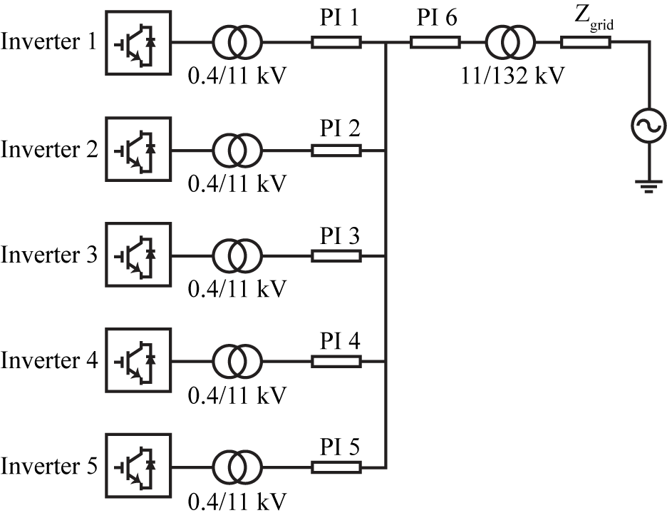
Figure 6 – Solar Farm Layout
| Cable | Length (km) | R (Ω) | L (H) | C (µF) |
|---|---|---|---|---|
PI1 | 0.31 | 0.04 | 1.273E-4 | 0.152 |
PI2 | 0.70 | 0.09 | 2.865E-4 | 0.345 |
PI3 | 1.07 | 0.14 | 4.138E-4 | 0.523 |
PI4 | 1.44 | 0.19 | 5.411E-4 | 0.704 |
PI5 | 1.64 | 0.21 | 6.366E-4 | 0.805 |
PI6 | 2.00 | 0.08 | 2.690E-4 | 0.620 |
5. Performance of thevenin equivalent model used together with the cable network
Although the Thevenin harmonic equivalent circuit parameters of a single inverter were initially used without considering any external cables, there is no certainty that such equivalent circuits will replicate the true harmonic behaviour when the actual inverters are used together with external cable networks. Hence, for the purpose of comparison of the individual performance, two cases were considered: (a) EMT model of the entire solar farm where each inverter is represented by an individual EMT model together with the external cable network (b) model of the entire solar farm of which each inverter is represented by the previously derived harmonic Thevenin models together with the external cable network.
As a part of this study, a single inverter was connected to the grid with the corresponding inverter cable (PI1, PI2, PI3, PI4 or PI5) and the cable between the 11 kV bus bar and the grid transformer (PI6) thus, giving five combinations. For instance, Inverter 1 is connected to the grid via an inverter transformer, corresponding inverter cable (PI1 cable) together with PI6 cable (giving a total cable length of 2.31 km) and the grid transformer. For each grid-connected inverter, the current harmonics at the PCC were extracted from the current injected into the grid. In order to determine up to what extent the Thevenin model can replicate the harmonic currents injected by an actual inverter, the same procedure was repeated, replacing the inverter EMT model with the Thevenin equivalent circuits of which the parameters are given for each harmonic order in Table 2. This analysis was carried out for 5th, 7th, 11th and 13th harmonics, which are the most significant harmonics in three-phase inverters. The outcomes of this study are shown in Figure 7. For the purpose of comparison associated with the influence of the cable network, the same test was repeated without the solar farm cables and the corresponding results correspond to ‘0’ on the abscissa. With the EMT models of inverters, the harmonic currents at the PCC are seen to decrease with increasing cable lengths of the system. Taking these as reference values, the absolute error associated with the harmonic currents measured, when the corresponding Thevenin models are operating, are shown in Figs. 6 (b), (d), (f), and (h). It is seen that although 5th and 7th harmonic currents are underestimated when the Thevenin models are used, the associated error can be accepted for practical purposes. For the 11th harmonic current variation predicated by the two approaches illustrate contradictory behaviours and also illustrated an unacceptable error as the cable length increases. For the 13th harmonic current, although the trends predicted by the two approaches are similar, the error associated is unacceptable as for the 11th harmonic current. It is crucial that these significant deviations are closely examined, which is undertaken below as it is expected that the vendor provided Norton/Thevenin harmonic models are expected to represent the behaviour of the actual inverters under reasonable and known inverter operating conditions.
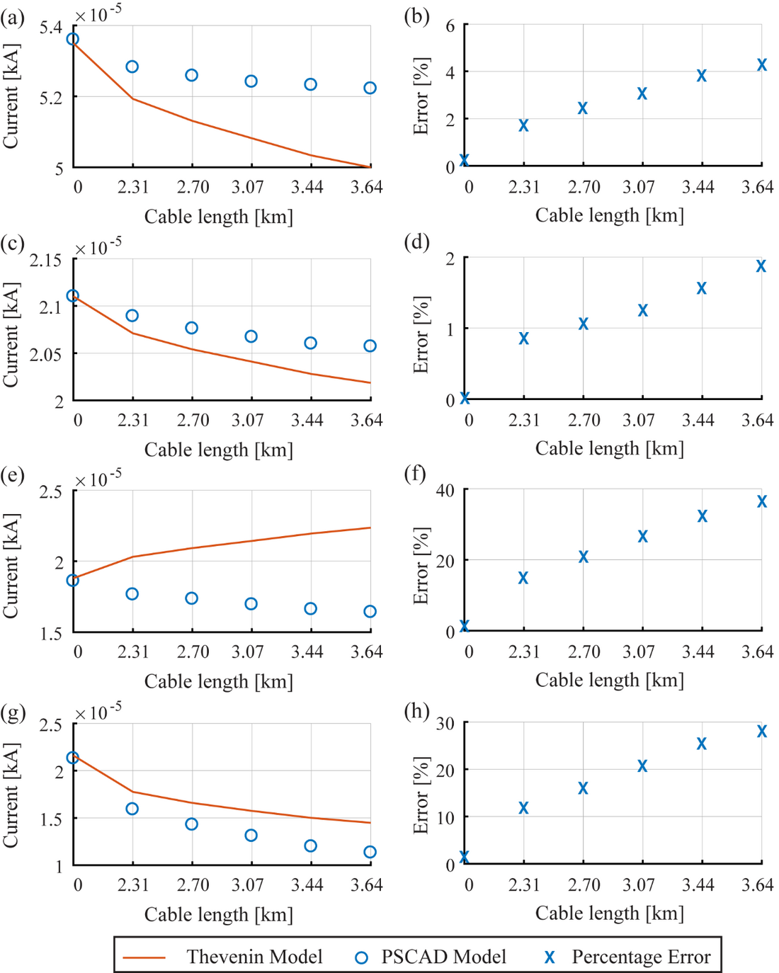
Figure 7 - Harmonic current magnitudes at the PCC with different cable lengths and their differences (a) 5th harmonic current (b) Percentage error for 5th harmonic current (c) 7th harmonic current (d) Percentage error for 7th harmonic current (e) 11th harmonic current (f) Percentage error for 11th harmonic current (g) 13th harmonic current (h) Percentage error for 13th harmonic
5.1 Analysis of the Results
Noting that the harmonic current emission behaviour of an inverter can be impacted by impedance variations external to the inverter, e.g. possible resonant conditions, impedance scans were undertaken at the inverter output terminals for both inverter 1 and inverter 5 (they are associated with the shortest and the longest cable lengths) respectively, employing both EMT models of the inverters and Thevenin models already developed (Table 2). Figure 8 illustrates the various impedance scans, where Figure 8 (a) represents the impedance scan of the system external to the output terminals of the EMT inverter model indicating an inductive behaviour. Noting that the 5th and 7th harmonic Thevenin impedances are also inductive, no resonant conditions are expected with the network external to the inverter system. As an example, with the 5th harmonic Thevenin impedance connected in series with the external network, the impedance scan obtained shown in Figure 8 (b) confirms that. This, therefore explains the decrease of the 5th and 7th harmonic currents as the cable length increases.
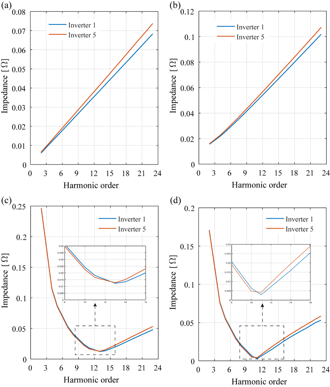
Figure 8 - Impedance scans (a) conducted at the output terminals of the inverter EMT model (b) with the 5th harmonic Thevenin impedance (c) with the 11th harmonic Thevenin impedance (d) with the 13th harmonic Thevenin impedance
Impedance scans undertaken with the 11th and 13th harmonic Thevenin impedances (that are both capacitive) connected in series with the external network demonstrate series resonant conditions as seen in Figures 8(c) and 8(d) where the series resonant frequencies are seen to lie within 9th and 15th harmonic. The increase in 11th harmonic current with increasing cable length (a dominant increase in capacitance rather than inductance) can be attributed to the movement of the resonance point closer to the 11th harmonic and the associated reduction in the net impedance. On the contrary, with regard to the decrease of the 13th harmonic current with increasing cable length (dominant increase in capacitance rather than inductance) can be attributed to the movement of the resonance point away from the 13th harmonic and the associated increase in the net impedance. These observations are based on close considerations given to the associated numerical calculations rather than on visual observation of the impedance scans only.
5.2 Critical Remark
Although the observations associated with various harmonic current variations can be unique to the present case considered, this study shows some limitations associated with the use of Thevenin equivalents in the place of appropriate inverter models that can represent the true harmonic behaviour. In summary, the interaction of Thevenin equivalent circuits (and their parameters determined in isolation) with the external system parameters that are used in harmonic studies may lead to unexpected behaviours such as resonances and hence due attention has to be paid.
6. Summation laws applied to the solar farm
With regard to multiple harmonic sources connected to a common point, considering their diversity, it is a common practice to apply the general summation law prescribed in IEC TR 61000.3.6 as given in (6)
(6)
where, Uh is the total current/voltage of hth harmonic order at the PCC; N is the number of harmonic sources connected to the PCC; Uhi is the hth harmonic voltage/current generated by the ith source. The α values are defined as follows.
It is also possible to apply arithmetic summation if there is no diversity between the harmonic sources (α=1 for all harmonic orders). In this part of the study, the solar farm model was used to test the validity of the application of the arithmetic and general summation law employing both EMT and Thevenin equivalent models to determine the resultant harmonic current levels at the PCC. Figure 9 (a), (c), (e) and (g) illustrate the observations derived considering 5th, 7th, 11th and 13th harmonics in relation to the following cases:
- EMT models of the individual inverter systems are added one by one in parallel, observing the harmonic current emission levels of the inverters at the PCC for each case. In Figure 9, these results are given as ‘simulation results’.
- EMT model of the individual inverter systems is considered one at a time observing harmonic current emission levels of the inverter and that at the PCC with a view of determining the resultant harmonic current levels at the PCC using arithmetic summation (approach 1) and general summation law (approach 2)
- Thevenin models of all inverter systems considered at the same time observing the resultant harmonic current levels (approach 3)
Considering the case where the resultant harmonic current levels were determined solely using the EMT models as the reference (simulation results), the error levels associated with the other three approaches given above are shown in Figure 9 (b), (d), (f) and (h).

Figure 9 - Comparison of the net harmonic currents at the PCC established using different approaches - low order harmonics
In addition to the low order harmonics considered above, studies were extended to cover higher-order 29th and 31st harmonics as well. These harmonic orders were chosen arbitrarily, where the study outcomes are shown in Figure 10.
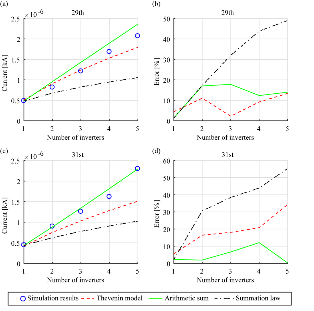
Figure 10 - Comparison of the net harmonic currents at the PCC established using different approaches - high order harmonics
6.1 Analysis of the results
From the results illustrated in Figure 9, it is evident that except for the 11th harmonic, the other harmonic current levels at the PCC tend to agree with arithmetic summation of the individual harmonic currents as evident from acceptable error levels. The application of the general summation law has led to results which are significantly inferior even when compared with the results obtained using the Thevenin models.
With the 11th harmonic, as the number of connected inverters grew from one to five employing the EMT models, it was noted that each new connection led to an approximately linear increase in the 11th harmonic currents of all the already connected inverters to a new, nearly equal level, whereas this was not the case with regard to other harmonics considered. This individual inverter behaviour at the 11th harmonic can be easily related to the collective trend illustrated by the resultant current at the PCC. This trend was also noted in the variation of the 11th harmonic voltage at the PCC.
The distinct difference in the case of the 11th harmonic requires detailed studies as it involves a multi-inverter scenario, combined with the solar farm cable network and the supply system. In addition, there is also the possibility of some harmonic amplification leading to harmonic currents that exceed simple arithmetic summation. Considering these possibilities, a relatively simplistic study hypothesising possible resonance conditions was undertaken by carrying out impedance scans at the terminals of one inverter as the other inverters were added to the network one by one. It is however to be noted that such impedance scans require all active 11th harmonic sources are short-circuited in the network. This approximate study was conducted at one of the inverter output terminals with the cables associated with each inverter introduced one by one, but the corresponding inverters removed while the supply network connected. This scan represents any resonance conditions associated with the cable network. These impedance scans clearly demonstrated series resonance conditions at around the 11th harmonic, thus supporting a corresponding increase in the 11th harmonic current as the number of inverters connected was increased. As an example, Figure 11 gives the outcomes of the impedance scan at one inverter terminal considering the network containing the cable network of three inverters together with the supply system, which clearly shows the series resonance conditions at around 11th harmonic.
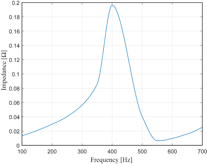
Figure 11 - Impedance scan conducted at one inverter terminal with a part of the cable network and supply system connected
6.2 Discussion
From the results in Figure 9 and Figure 10, it can be concluded that the arithmetic summation of the individual inverter harmonic currents, except for the 11th harmonic are in close agreement with the resultant harmonic currents measured at the PCC using the EMT models. The arithmetic summation of the individual inverter harmonic currents predicted using the Thevenin equivalent circuits also demonstrated a promising outcome. However, as expected, the actual inverter harmonic currents will be dependent on the external network.
7. Conclusion
The paper described the application of the commonly known small-signal technique for the determination of Thevenin/Norton equivalent circuits of large-scale inverters that are used in solar farms with a view to examine the validity/limitations of their use in harmonic studies, noting that such circuits are provided by inverter manufacturers/vendors. The accuracy of the derived Thevenin/Norton models was tested using EMT models where good agreement was observed, but with the limitation that the harmonic behaviour predicted by such models will be subjected to varying conditions of the network external to the inverters. One of the main influencing factors noted in this study was the network resonance conditions which can arise together with the Thevenin/Norton impedances thus affecting the true harmonic behaviour as predicted by EMT models. Although not examined in the work undertaken, the resonance conditions associated with the external grid can also affect the harmonic performance predicted using Thevenin/Norton models and hence care is required in identifying the root cause for discrepancies that can arise when compared with true harmonic behaviour predicted by the EMT models. The work presented also demonstrated that arithmetic summation of individual inverter harmonic currents is in reasonable agreement with the actual resultant harmonic current but care is required as above network behaviours (resonance conditions) can lead to violation of the simple arithmetic summation of the individual currents. The general conclusion of this study is that, although Thevenin/Norton models are commonly used in harmonic studies, care is required in their application. It is also to be noted that the Thevenin/Norton models developed are subjected to significant variabilities depending on the operating power levels adding further difficulties to their application in real life.
References
- J. Smith, S. Ronnberg, M. Bollen, J. Meyer, A. Blanco, K.-L. Koo, and D. Mushamalirwa, “Power quality aspects of solar power– results from cigre JWG C4/C6.29,” CIRED-Open Access Proceedings Journal, vol. 2017, no. 1, pp. 809–813, 2017.
- M. Ayub, C. K. Gan, and A. F. A. Kadir, “The impact of grid connected PV systems on harmonic distortion,” in 2014 Innovative Smart Grid Technologies - Asia (ISGT ASIA), 2014, pp. 669–674.
- J. Arrillaga and N. R. Watson, Power system harmonics. John Wiley & Sons, 2004.
- Operational Analysis and Engineering, AEMO, Power System model guidelines. AEMO, 2018.
- International Electrotechnical Commission, “Electromagnetic compatibility (emc)–part 3-6: Limits–assessment of emission limits for the connection of distorting installations to MV, HV and EHV power systems,” Int. Electro technical Commission, Geneva, Switzerland, IEC/TR 61000-3-6, 2008.
- H. Moghadam, F. Ackermann, and S. Rogalla, “Improving the summation law for harmonic current emissions of parallel operated PV inverters by considering equivalent grid impedance,” in Int. Conf. on Renewable Energies and Power Quality, Spain, 2017.
- F. Medeiros, D. C. Brasil, P. F. Ribeiro, C. A. G. Marques, and C. A. Duque, “A new approach for harmonic summation using the methodology of IEC 61400-21,” in Proceedings of 14th International Conference on Harmonics and Quality of Power - ICHQP 2010, 2010, pp. 1–7.
- A. D. Rajapakse and D. Muthumuni, “Simulation tools for photovoltaic system grid integration studies,” in 2009 IEEE Electrical Power Energy Conference (EPEC), 2009, pp. 1–5.
- R. Pena-Alzola, M. Liserre, F. Blaabjerg, M. Ordonez, and Y. Yang, “Filter design for robust active damping in grid-connected converters,” IEEE Transactions on Industrial Informatics, vol. 10, no. 4, pp. 2192–2203, 2014.
- R. Teodorescu, M. Liserre, and P. Rodriguez, Grid converters for photovoltaic and wind power systems. John Wiley & Sons, 2011.
- A. Yazdani and R. Iravani, Voltage-sourced converters in power systems: modeling, control, and applications. John Wiley & Sons, 2010.
- A. Sangwongwanich, A. Abdelhakim, Y. Yang, and K. Zhou, “Chapter 6 - control of single-phase and three-phase dc/ac converters,” in Control of Power Electronic Converters and Systems, F. Blaabjerg, Ed. Academic Press, 2018, pp. 153–173.
- A. M. Vural, “PSCAD modeling of a two-level space vector pulse width modulation algorithm for power electronics education,” Journal of Electrical Systems and Information Technology, vol. 3, no. 2, pp. 333–347, 2016.
- K. Zhou and D. Wang, “Relationship between space-vector modulation and three-phase carrier-based PWM: a comprehensive analysis [three-phase inverters],” IEEE Transactions on Industrial Electronics, vol. 49, no. 1, pp. 186–196, 2002.
- J. Sun, “AC power electronic systems: Stability and power quality,” in 2008 11th Workshop on Control and Modeling for Power Electronics, 2008, pp. 1–10.
- J. Sun, “Small-signal methods for ac distributed power systems – a review,” IEEE Transactions on Power Electronics, vol. 24, no. 11, pp. 2545–2554, 2009.
- J. Arrillaga, B. C. Smith, N. R. Watson, and A. R. Wood, Power system harmonic analysis. John Wiley & Sons, 1997.
- A. Bosman, J. Cobben, J. Myrzik, and W. Kling, “Harmonic modelling of solar inverters and their interaction with the distribution grid,” in Proceedings of the 41st International Universities Power Engineering Conference, vol. 3, 2006, pp. 991–995.
- E. C. Aprilia, V. C´uk, J. F. G. Cobben, P. F. Ribeiro, and W. Kling, “Modeling the frequency response of photovoltaic inverters,” in 2012 3rd IEEE PES Innovative Smart Grid Technologies Europe (ISGT Europe), 2012, pp. 1–5.
- S. Rogalla, F. Ackermann, N. Bihler, H. Moghadam, and O. Stalter, “Source-driven and resonance-driven harmonic interaction between PV inverters and the grid,” in 2016 IEEE 43rd Photovoltaic Specialists Conference (PVSC), 2016, pp. 1399–1404.
- A. Robert, T. Deflandre, E. Gunther, R. Bergeron, A. Emanuel, A. Ferrante, G. Finlay, R. Gretsch, A. Guarini, J. G. Iglesias et al., “Guide for assessing the network harmonic impedance,” in 14th International Conference and Exhibition on Electricity Distribution. Part 1. Contributions (IEE Conf. Publ. No. 438), vol. 2, 1997, pp. 3/1–310.
- T. J. Browne, Harmonic management in transmission networks. Ph.D. Thesis, University of Wollongong, 2008.
- CIGRE Working Group B1.30, Cable Systems Electrical Characteristics. CIGRE, 2013.
- Olex, Nexans Olex High Voltage Cable Catalogue. Nexans Company, 2009.