Pattern recognition based protection schemes for power transmission lines
A. VALABHOJU - PhD Student
A. YADAV - Supervisor
National Institute of Technology Raipur, India

Summary
Topologically speaking, power system network is the widest and complex interconnected network in service expanded through different geographical territories. In recent days power system network is frequently exposing to various types of disturbances and creating thought-provoking engineering challenges. The transmission line is the most vulnerable of the power system network due to its very large physical size. Among the various systems designed to protect the components of different power systems, protecting transmission lines is a major challenge. Thermal, electrical, mechanical and environmental pressures are a major cause of fault (or) disruptions in transmission lines that can be grouped together as common shunt fault (CSFs), multi-location shunt faults (MLFs) and evolving faults (EVFs). In general, most existing standard transmission systems do not work well in cases of abnormal faults such as MLFs and these MLF is defined as a Cross-country fault (CCF) occurring at different phases of the same circuit at different location at the same or different time. Evolving faults (or) Transforming faults occur when a single phase/line fault is converted into a double or triple line fault after some time delay in the same location or in a different location. Proper protection system should be designed to detect a fault, if not detected, that could lead to equipment damage or long-term loss of service and reduce the resilience / reliability of the power system [1].
Nowadays, new attention has been given to develop protective relaying schemes using Artificial Intelligent and advanced signal processing techniques. In this research work, novel relaying algorithms/schemes have been designed for detection, classification and location of CSFs, MLFs and EVFs for a large utility system i.e., real power transmission network of Chhattisgarh state as research of interest. Primarily, this comprehensive research work is comprising of four stage process; In first stage, modelling and simulation of 400kV, 50Hz, Chhattisgarh state power transmission (CSPT) network in MATLAB/Simulink software and RSCAD/RTDS environment using the actual network data/parameters collected from local power transmission utility (CSPT). In second stage, pilot studies such as load flow studies and short circuit studies are carried out to replicate atypical fault scenarios on a double-circuit transmission line (DCTL) of CSPT network. Further extensive simulation studies have been performed to reproduce different type of fault event records (data sets) by varying fault parameters such as fault resistance (Rf), fault inception angle (ϕf ), and fault location (Lf). In third stage, design/development of novel relaying algorithms/schemes by using different artificial intelligent techniques and advanced signal processing techniques for detection, classification and location of CSFs, MLFs and EVFs. Furthermore, the performance of proposed/designed relaying schemes have been investigated in presence of measuring noise and effect of CT saturation/CCVT transients. Additionally, exclusive case studies have been carried out to evaluate the performance of proposed/designed relaying algorithms at no-fault dynamic/stressed conditions to investigate the impact of high-impedance faults (HIF), power swing (PS) and load encroachment conditions etc. In Fourth stage, validation of proposed/designed relaying schemes have been done with real-time data such as actual field fault data and real-time data generated in RSCAD/RTDS environment. Besides that, few case studies have been performed on a prototypical model of 180km transmission line in the laboratory environment to confirm the adaptability/applicability of proposed/designed relaying schemes for practical power system network.
Finally, to determine efficacy of proposed/designed relaying schemes a thorough analysis and assessment of results have been done thereby calculating/comparing of performance metrics and error metrics. Furthermore, to benchmark the research outcomes of this work, comparative assessment has been carried out for proposed/designed relaying schemes individually with existing (or) previously reported relaying schemes. Moreover, the proposed/designed relaying schemes and their outcomes are confirming the adaptability and applicability in practical power transmission system to improve reliability and stability. The implementation of proposed/designed relaying schemes can help the line patrolling crew in restoration of power supply by attending/clearing the fault as early as. The outcomes of this project work can give research insights to the protection engineers/researchers and also useful to the local power utilities.
However, to improve the fault diagnostic capabilities different relaying schemes/algorithms were designed and reported in various national/international journals and conferences during the execution of this research work. Few of the most remarkable research objectives are cited below and corresponding methodology/results have been elaborated in further sections 1 to 5:
1. A real-time protection algorithm/scheme for detection/classification of CSFs during power swing (PS)
In this section, Maximal Overlap Discrete Wavelet Transform (MODWT) is used to extract features from current signals during stable PS condition. MODWT is a modified form of Discrete Wavelet Transform (DWT) and is often used for real-time fault analysis and other power system disturbance studies [2-4]. The standard deviation (SD) values of the MODWT coefficients of the current signals are used only as input features for fault detection (FD) and fault classification (FC). The proposed scheme is based on a three-dimensional fault triangle (3DFT) with different fault planes. The performance of the proposed scheme has been evaluated with real-time field failure data using the 'Wavewin' software environment.
1.1. Proposed relaying scheme based on MODWT
The proposed protection scheme employs in two-segment process as demonstrated in Fig.1 and the segment-I is associated with the FD scheme. Initially, the MODWT has been implemented to current signals and. The FD scheme has been performed through the real-time analysis of SD values of wavelet coefficients of current signals [5]. In the segment-II, categorizes the type of fault in real-time soon after the detection of CSFs in the segment-I and all types of CSFs are classified based on the normalized SD values by projecting post fault samples on 3DFT.
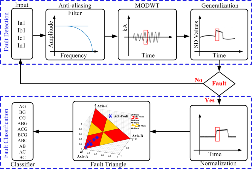
Figure 1 - Block diagram of proposed scheme based on MODWT [5]
a. Fault Detection (FD) scheme for CSFs during PS
A stable PS is originated by inception of a three-phase to ground fault on the next line associated to the monitored bus (bus-4) and clearing the same fault before the critical clearing time (CCT). For instance, a three-phase to a ground fault has been incepted at 1.001s on a single circuit transmission line of 60 km length which is connected between bus-4 (KSTPC/NTPC) & bus-11(Sipat) [5] and the same has been cleared by tripping the circuit breakers of both the ends at 1.15s which initiated a stable PS scenario in the transmission network. Extensive simulation has been performed thus creating a different type of CSFs during steady PS to design a real-time algorithm to detect and classify faults at a fixed time (Ts) = 1.0ms (sampling frequency fs = 1.0 kHz). Typically, Digital Fault Recorder (DFR) are pre-configured to 1.0kHz and 1.2kHz frequencies. This sample frequency is sufficient to find the appropriate attributes of the signals in the pre-processing phase data and proceed to calculate the wavelet coefficients of the phase / neutral currents in each / every simulation event without delay. The frequency band of the wavelet coefficients will decrease at each level / throughout the decomposition. Significantly, the coefficients of wavelength in the 2nd decomposition level are defined as the appropriate feature to investigate the components of an exaggerated frequency signal. The feature of faulty signals can be detected by analysing their temporary nature at the instant of fault inception. Since the faulty signal is divided into wavelet coefficient on different scales, faulty signal attributes can be detected by investigating the wavelet coefficient in the accurate time scale, especially these wavelet coefficients are often exaggerated by the frequency-transient components. In this context, the fault is detected in real time, sample by sample, using a recursive window (full-cycle) of current signal during the stable PS. All types of CSFs can be detected in real-time, sample by sample at a given time, the SD values of the MODWT coefficients are calculated in the full-cycle window using eqn. (1-4) as follows:
(1)
(2)
(3)
(4)
Where ‘k’ is the current sample, ‘i’ is the sample count, ‘N’ is the total number of samples, μ is the mean of the samples, wiA(k), wiB(k), wiC(k), wiN(k) are the MOPDWT coefficients of three-phase currents and neutral current sample, σiA(k), σiB(k), σiC(k), σiN(k) are SD values of three-phase/neutral currents respectively.
b. Fault classification (FC) scheme for CSFs during stable PS
All type of CSFs during stable PS are categorized in real-time, sample by sample using a recursive window (full-cycle) after post-fault instant. The SD values of the MODWT coefficients are standardized to calculate the fault coordinates using eqn. (5-8) in a full-cycle window over a period of time. Normalized SD values after post-fault instant are projected on the generalized 3DFT to classify different types of CSFs.
(5)
(6)
(7)
(8)
Where A(s), B(s), C(s), G(s) are the fault coordinates of three phase(s) and neutral currents, σiA(k), σiB(k), σiC(k), σiN(k) are the SD values of three-phase(s) and neutral currents respectively.
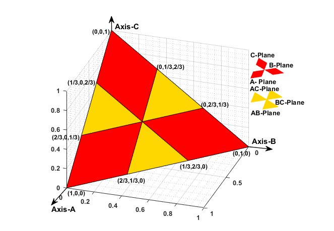
Figure 2 - Fault triangle with different fault planes [2-5]
To categorize different types of CSFs during stable PS, fault classification (FC) protocols have been demarcated followed by a 3DFT [5]. These FC protocols have demarcated by calculating fault co-ordinates where the SD values of MODWT coefficients are normalized using eqn. (5-8). If the normalized SD value exceeds the pre-configured threshold, then the fault patterns are classified/projected in the respective sub-plane/region demonstrated in Fig. 2. The 3DFT has been strategized by considering three perpendicular axes with equal length (1- unit) where each axis represents a coordinate of a 3DFT such as axis-A denotes Phase-A1, axis-B denotes Phase-B1 and axis-C denotes Phase-C1. The normalized SD values of full-cycle data (post fault instant) are projected on a 3DFT plane. Subsequently, fault sub-plane/regions have been demarcated for different type of fault such as A-plane, B-plane, C-plane for single-phase-to-ground faults and AB-plane, BC-plane and CA-plane for phase-to-phase and double-phase to ground faults.
1.2. Case studies with results and discussion
The MODWT based real-time algorithm has been critically assessed by performing simulation studies to determine the CSFs, and faulty phase(s) of DCTL during stable PS condition. The performance of proposed relaying scheme has been evaluated for different fault/operating scenarios such as variation in fault parameters, effect of CT saturation and CCVT transients, variation in operating voltage / frequency / source impedance / sampling frequency / signal-to-noise ratio (SNR) etc. Fig.3 demonstrates a case study of fault during stable PS with variation in operating voltage.
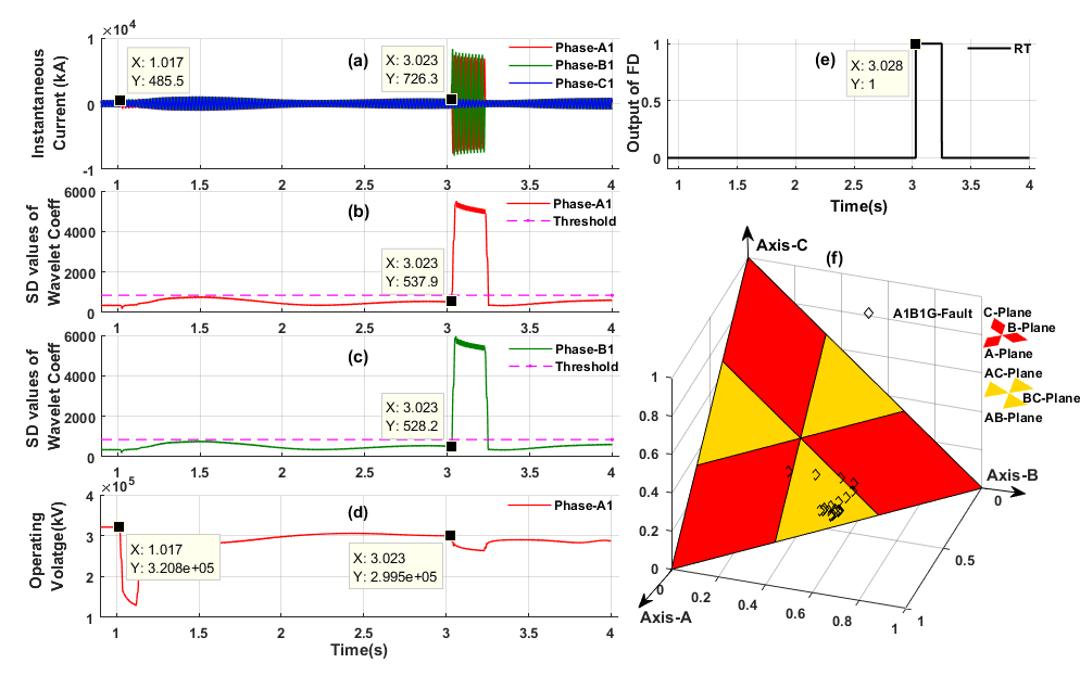
Figure 3 - Demonstration of proposed scheme for A1B1G fault during stable PS with variation in operating voltage: (a) three-phase currents (b) SD values of MODWT coefficients of phase-A1 (c) SD values of MODWT coefficients of phase-B1 (d) Operating voltage at sending-end bus (NTPC/KSTPS) (e) trip signal of FD scheme (f) projection of FC scheme [5]
The proposed MODWT-based scheme has been tested with real-time field fault events recorded by the DFR at bus 4 (NTPC/KTPS) of 400kV, 50 Hz, existing CSPT network of India. The time, day and year of the events occurred in different sub-stations of Chhattisgarh state power transmission company Ltd. (CSPTCL), as recorded by DFR are given along with the detection time by the proposed scheme and the type of fault occurred with or without power swing [5]. Moreover, the proposed MODWT-based relaying scheme detects and classifies all types of CSFs during stable PS with a minimum 0.05 cycle to maximum 0.5-cycle response time precisely. The performance was also evaluated for real-time field fault data recorded by DFR in a sub-station of an Indian power system utility (CSPT) and test results are noticeable.
2. Advanced fault detection and classification scheme for CCFs and EVFs
In this section, MODWT has been employed to extract the characteristics of the faulty-signals in case of CCFS and EVFs. These CCFs and EVFs are exhibits complex in nature and should be detected as early as [6-7]. The max. change in wavelet energy of 3-phase currents is identified as the unique feature for detection/classification of CCF&EVFs. The performance of the proposed scheme has been tested in real-time digital simulator (RTDS) laboratory and also validated the same on a prototypical model of transmission line in the laboratory setup.
2.1. Proposed protection scheme based on MODWT for detection and classification of CCFs and EVFs
The proposed protection scheme includes the 3-stage method as demonstrated in Fig.4 and the stage-I includes data pre-processing and feature extraction followed by the real-time FD scheme is employed in the stage-II and in the stage-III FC scheme has been executed. In stage-I, the MODWT is implemented to 3-phase instantaneous currents and corresponding wavelet coefficients are computed at scale-2 using “fk6” as mother wavelet function [8]. The fault detection scheme is carried through the real-time analysis of the wavelet energy values of wavelet coefficients in stage-II. The stage-III employs classification of CCFs and EVFs through normalization of wavelet energy values in real-time.
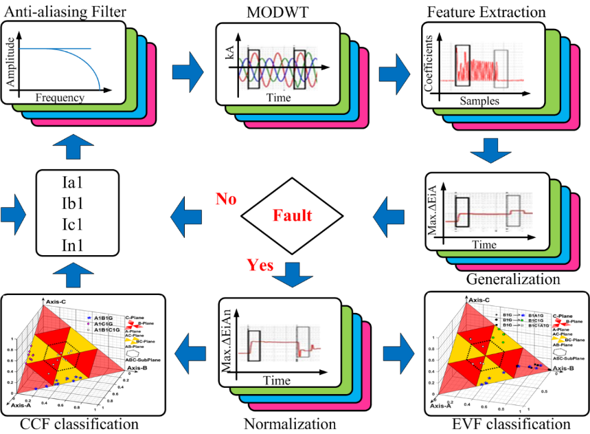
Figure 4 - Block diagram of proposed scheme based on MODWT for CCFs/EVFs [8]
a. Fault Detection (FD) scheme for CCFs & EVFs
To replicate actual fault scenarios, an existing 400kV 50 Hz, CSPT network has been modelled in RSCAD/RTDS software setup, data of the same network is cited in [8] and different types of CCFs and EVFs have simulated with ts=50μs (sampling frequency fs=20 kHz). The sampled phase/neutral currents are taken into account to calculate the wavelet energy values of the MODWT coefficients. The nature of faulty signals can be identified through analysis of their transient nature at fault instant. Since the voltage/current signal is decomposed into wavelet coefficients at different scales, the nature of the signals can be determined by investigating the wavelet coefficient on a precise time scale, predominantly these wavelet coefficients are often exaggerated by the frequency components of the fault-induced transients. In this context, the fault is detected in real-time, sample-by-sample, by computing the max. change in MODWT energy of current signal in a ½ -cycle window. In each/every simulation a recursive window (½ -cycle) has considered as a frame in such a way that the number of frames is equal to the number of samples of a faulty signal as mentioned in eqn. (9-12). The max. change in MODWT energy of current signal in a ½ -cycle window is computed as follows:
(9)
(10)
(11)
(12)
Where ‘k’ is the current sample, ‘∆k’ is the window size and ∆EiA, ∆EiB, ∆EiC, ∆EiG are the change in MODWT energy of corresponding phase and neutral current signals.
b. Fault Classification (FC) scheme for CCFs & EVFs
For FC scheme, the change in wavelet energy has been normalized using eqn. (13-16) to calculate the fault coordinates. These fault coordinates have been calculated by through the normalization of max. change in wavelet energy in a recursive window (½-cycle) and defined a general threshold set value, and then the faulted samples are projected on the respective fault plane of a generalized three-dimensional fault plane (G3DFP) to identify the corresponding fault-plane for classification of CCFs/EVFs.
(13)
(14)
(15)
(16)
For classification of different CSFs, CCFs and EVFs, a G3DFP as illustrated in Fig. 5(a). It is an amalgamation of three-dimensional triangular plane and hexagonal planes considering three perpendicular axes with equal length. The triangular fault plane shown in Fig. 5(b) is for CSFs and hexagonal fault plane shown in Fig. 5(c) is for CCFs/EVFs. The fault coordinates of this G3DFP representing the three axes as the three phases A, B, and C of the transmission line have been calculated using equations (13-15) respectively. According to eqn. (16), presence of ground fault (G) has been distinguished. Moreover, fault coordinates have been calculated for different fault planes/sub-regions such as phase-to-ground and phase-to-phase faults.
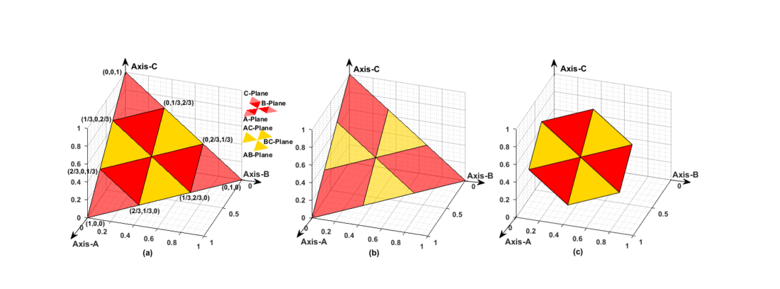
Figure 5 - Fault Classification Plane:(a) G3DFP (b) Triangular fault plane for CSFs (c) Hexagonal fault plane for CCFs/EVFs [8]
2.2. Case studies with results and discussion
Rigorous simulation studies have been carried out to examine the proposed MODWT based protection scheme. Simulation studies of different fault events are carried out in RSCAD/RTDS environment and measured voltage/current signals of the sending-end bus-B4 (NTPC/KSTPS) are used for testing of proposed MODWT based relaying scheme. Several fault cases are simulated on DCTL of CSPT network, cited in [8]. Various fault conditions have been generated with the variations of different fault parameters and variation in operating voltage/frequency/load angle/sampling frequency/signal-to-noise ratio. Also, performance of proposed relaying scheme has been tested for effect of CT saturation, CCVT transients and stable PS condition etc. The potential of applicability of MODWT-based scheme has been evaluated by performing experiments of different CCFs and EVFs on a prototypical model of power transmission line of 180km length in the laboratory environment which replicates fault signal of real-time field fault data. The fault signals have been recorded by a DFR (Hall Effect Sensor-LV/LA-25P) with a combination of Data Acquisition Card (VUDAS-100) at a sampling frequency of 10 kHz. These recorded fault signals have been transferred through an ADC/DAC converter followed by a low-pass filter to the master control unit (PC) in which the MODWT-based scheme has been deployed to issue trip logic for FD scheme and FC scheme as well. Fig.6 shows the test results of a CCFs on an experimental setup in laboratory environment with fault parameters as Rf =0.001 Ω, Lf1=40 km, Lf2 =100 km, ϕf=30°. In this case also, the MODWT-based scheme has detected the CCFs within ½ cycle time successfully. Fig. 7 shows the performance validation with experimental data using a hardware setup in case of CCFs incepted at 2.252s and detected the same at 2.253s and classified the same fault on a G3DFP.
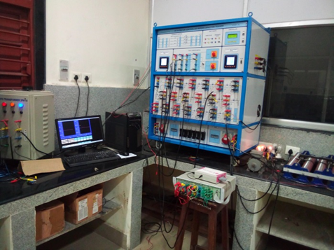
Figure 6 - A prototypical model of 180km transmission line connected with Hall-effect sensor [8]
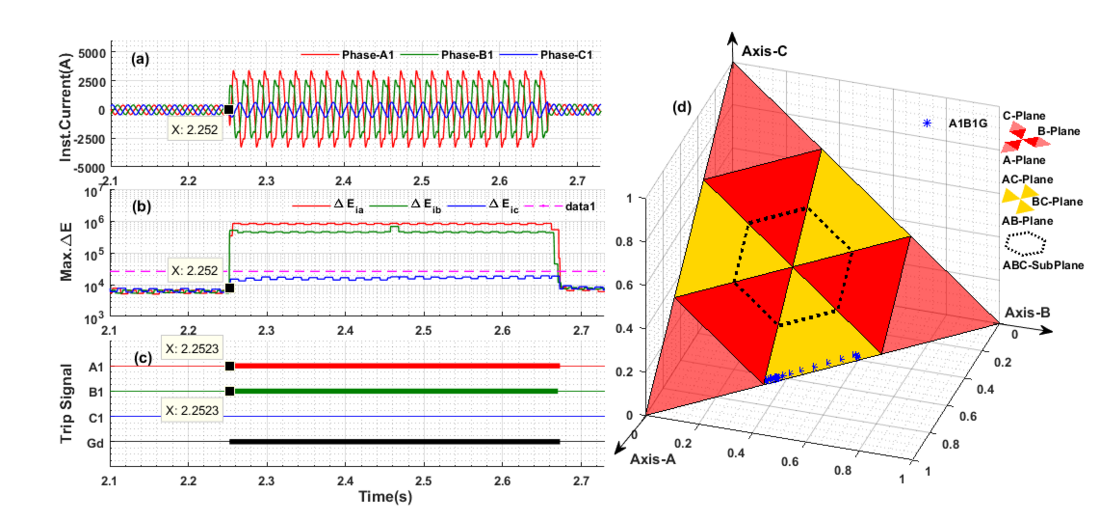
Figure 7 - Experimental validation of proposed scheme based on MODWT in case of CCFs: (a) Three-phase currents (b) Max. of change in MODWT energy of three-phase currents(c) FD scheme output (d) FC scheme output [8]
3. A new fault diagnosis scheme for detection and classification of CCFs and EVFs with emphasis on high-impedance fault (HIF) syndrome
In the modern power system network, transmission lines are subject to atypical fault scenarios. This transmission line is the longest component in the power system and sometimes passes through forest area where the formation of CCFs and EVFs associated with HIF syndrome (features) is frequent due to thunderstorms, cyclones and poor vegetation management and improper tree pruning. In this work, Maximal Overlap Discrete Wavelet Packet Transform (MODWPT) has been employed to extract the characteristics of the signals during CCFs with HIF (CCF-HIF) and EVFs with HIF (EVF-HIF) which are more complex and aperiodic/asymmetric/non-linear in nature. The max. change in wavelet packet energy (MWPE) of MODWPT coefficients of currents/voltages have been considered as the unique feature to design proposed scheme in a DCTL of CSPT network using MATLAB/Simulink.
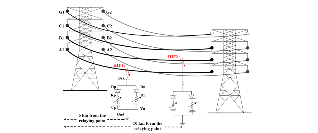
Figure 8 - CCFs with an ideal-HIF model in a DCTL [10]
Generally, the CCF-HIFs can be characterized as “high-impedance ground faults happening in diverse phases of the one circuit at different locations at same fault inception time”. For example, the Fig.8 illustrates a CCF with HIF syndrome initiated on phase ‘A1’ at 5km and phase ‘B1’ at 10 km in circuit-I of DCTL by using an ideal HIF model. Further Fig.9 demonstrates an EVFs with HIF syndrome which has occurred at 5km away from the relaying point while HIF1 incepted on phase-A1 at ϕt1=0.1s and HIF2 occurred on phase-B1 at ϕt2=0.14s. The detection of CCFs and EVFs with HIF is challenging task because the fault current magnitude is very low and it is asymmetric, non-linear and non-periodic in nature.
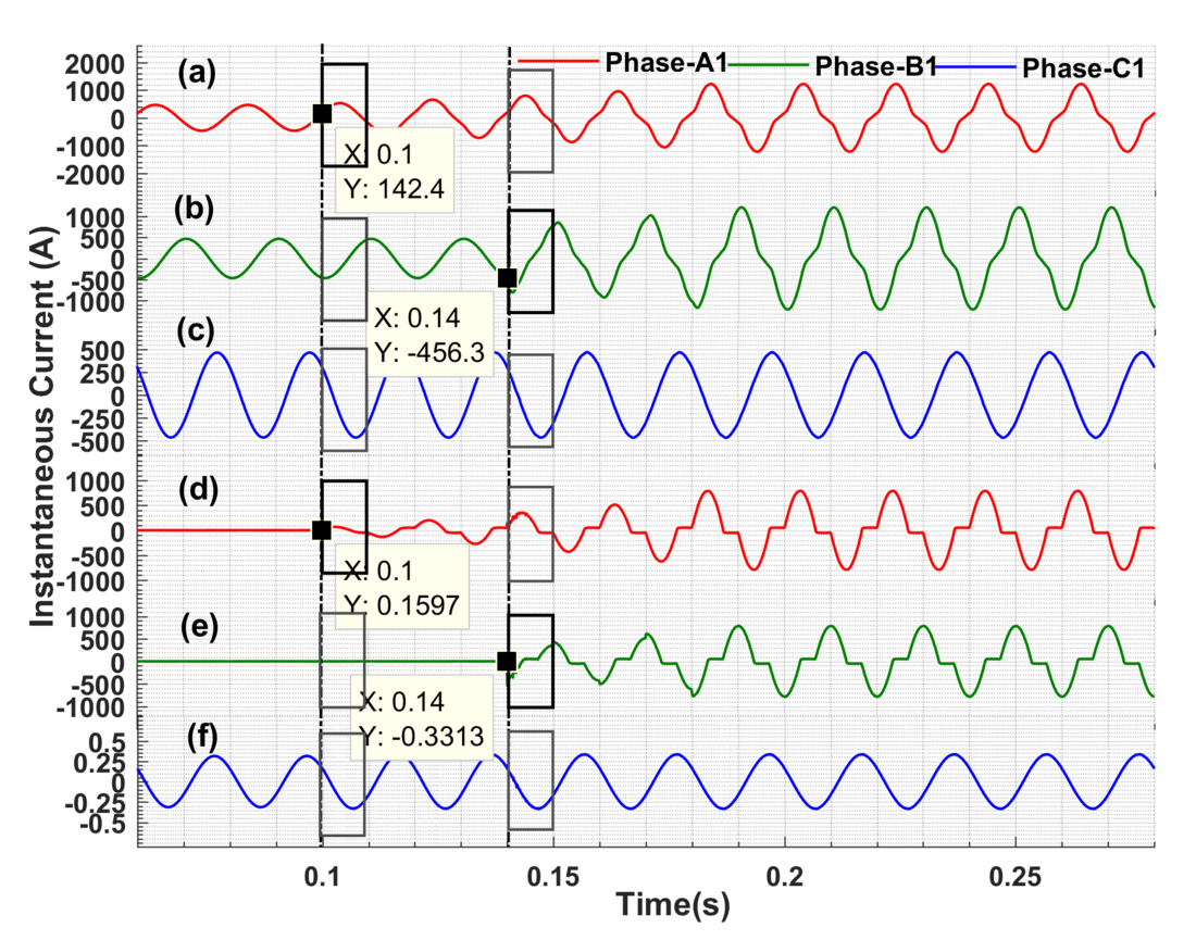
Figure 9 - A case study of the EVF with HIF syndrome: (a) Instantaneous current of phase-A1at sending-end (b) Instantaneous current of phase-B1 at sending-end (c) Instantaneous current of phase-C1 at sending-end (d) Instantaneous fault current of phase-A1 through HIF1 (e) Instantaneous fault current of phase-B1 through HIF2 (f) Instantaneous fault current of phase-C1 at HIF location
3.1. Proposed fault diagnosis scheme based on MODWPT
MODWT is suitable for real-time analysis through the extraction of transient features of faulty signal in time domain [9-10]. The investigation of frequency component in a specific time-scale is more suitable for aperiodic, asymmetric, non-stationary HIF signal [10]. In this context, the wavelet packet energy values (MWPE) at level-1 are calculated from MODWPT coefficients at each/every sample instantly. MODWPT splits the energy between wavelet packets at each decomposition level. The sum of the energy on all wavelet packets is equal to the total energy of the input signal. The result of MODWPT is useful for applications where analysis of energy levels in different packets can be used. The outputs of MODWPT detail coefficients are useful for applications that require time tuning, such as real-time analysis.
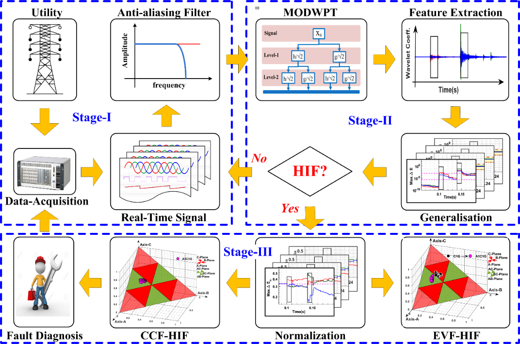
Figure 10 - Block diagram of proposed fault diagnosis scheme based on MODWPT [10]
Fault diagnosis scheme is executed in three stages illustrated in Fig.10 and the stage-I comprise data-acquisition from the network followed by pre-processing the voltage/current signal with the anti-aliasing filter. In the stage-II, mining of exclusive feature from voltages/currents signals by applying MODWPT and further generalization of threshold set, then the detection of CCFs/EVFs with HIF syndrome simultaneously [10]. Detection of HIF syndrome has been carried out simultaneously by computing the wavelet packet energy (MWPE) values at level-1/node-1 of MODWPT coefficients using eqn. (17-20) as follows:
(17)
(18)
(19)
(20)
Where ‘r’ is the sample count of the wavelet packet energy of MODWPT coefficients, ‘∆r’ is the window size, WiA, WiB, WiC, WiN are MODWPT detail coefficients of three phases : A, B, C and neutral currents correspondingly and EiA, EiB,EiC, EiN are the MWPE values of respective phase(s)/neutral currents. Normalization of max. change in MWPE has been done in a ½ cycle frame to classify all type of CCF-HIFs and EVF-HIFs on a three-dimensional fault plane (3DFP) at stage-III. Then the post-samples are plotted on corresponding fault-plane/sub-plane of a 3DFP which is an amalgamation of a triangular-plane and hexagonal-plane.
a. Detection of CCF-HIFs & EVF-HIFs
To reproduce HIF syndrome, 400kV, 50Hz, CSPT network has been modelled/simulated in MATLAB/Simulink [10] and various kinds of CCF-HIFs and EVF-HIFs are reproduced at a definite time, ts=50μs (sampling-time). Then after, the MODWPT detail coefficients are computed at different level/node. The HIF syndrome is detected simultaneously by calculating the max. change in MWPE of voltage/current signal in a ½-cycle frame. The no. of frames is identical to the no. of samples of a HIF-signal as defined in [10]. The change in MWPE of the current signals for each phase in a ½ -cycle frame is calculated using eqn. (21-24) as follows:
(21)
(22)
(23)
(24)
In the same way, the change in MWPE of voltage signals for each phase is computed using equation (25-27):
(25)
(26)
(27)
Where ‘r’ is the samples count, ‘∆r’ is the frame size and ∆EiA, ∆EiB , ∆EiC , ∆EiN are the change in MWPE values of respective current signals and ∆EvA , ∆EvB , ∆EvC are the change in MWPE values of respective voltage signals.
Energy Envelope Index (EEI)
Since the transients induced by HIF syndrome are over-damped, lasts long for many seconds or hours and marks mainly the fault currents, so the max. change in MWPE of the faulty phase increases moderately for long time (more than 5- cycle time) as such as the high-impedance object (H) is in touch with the live conductor [10]. Whereas in case of a CSFs(non-HIF), the max. change in MWPE of the faulty phase increases suddenly for a short time then after reaches to normal reference value as such a CSF will be cleared in zone-I within 2-3 cycle time (max. of 5-cycle). In view of the above, an energy envelope index (EEI) [10] has been defined as a generalized threshold to design the proposed protection scheme, thereby assuming two threshold indices such as upper threshold ( i1 and
v1) and lower threshold (
i2 and
v2) corresponding to currents and voltages respectively. Here “
i1” and “
v1” helps to discriminate HIF with other switching events and activates the proposed fault diagnosis algorithm and “
i2” and “
v2” aids to discriminate the HIF with CSFs/CCFs, since the max. change in MWPE of faulty-phases lies within the EEI because of the existence of HIF syndrome. In case of CSFs/CCFS the max. change in MWPE of faulty-phases at the fault instant suddenly rises above “
i2” and goes below “
v2” and will not lies within the EEI until the fault clears on the respective faulty phase(s). This proposed EEI has been generalized for numerous operating/switching conditions by performing extensive simulation studies with variation in diverse fault parameters.
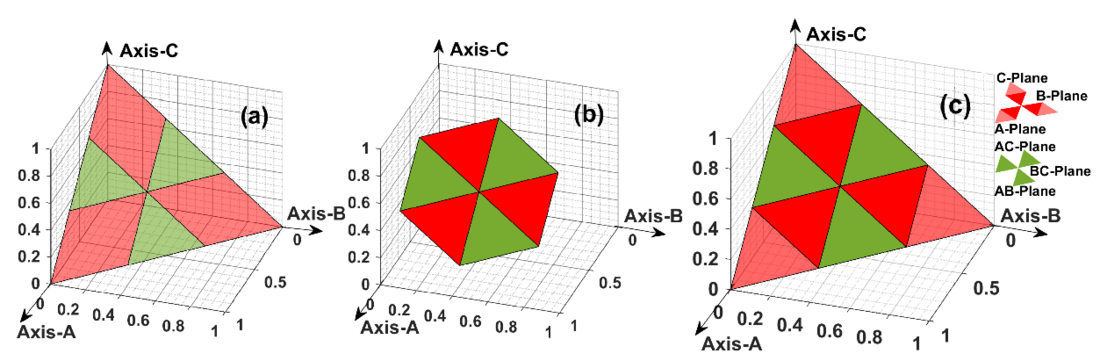
Figure 11 - Fault Classification Plane: (a) Triangular-plane for CSFs (HIF/non-HIF) (b) Hexagonal-plane for CCFs and EVFs with HIF/non-HIF (c) Normalized 3DFP [10]
b. Classification of CCF-HIFs & EVF-HIFs
For classification of (CCF-HIFs)/(EVF-HIFs), the max. change in MWPE has been normalized using eqn. (28-31) further to calculate the coordinates of fault-plane. The coordinates of fault-plane are computed based on eqn. (28-31) to find the corresponding fault-plane/sub-plane for classification. These HIFs are being classified by assessing the normalized values of max. change of MWPE in a ½ -cycle frame at a definite time with a predefined threshold set (c), and then after the post-samples are plotted on the corresponding fault-plane/sub-plane of a 3DFP demonstrated in Fig.11.
(28)
(29)
(30)
(31)
3.2. Case studies with results and discussion
The proposed fault diagnosis scheme is tested thereby simulating different fault cases on a DCTL of CSPT network by varying different parameters, i.e. fault type (ft ), fault location (Lf ), fault inception angle (f ), and fault resistance (Rf ). The proposed fault diagnosis scheme has been assessed with exclusive case studies including no-fault/dynamic conditions, also tested for effect due to switching of capacitor bank (CSW), switching of reactor strings (RSW), switching of loads/feeders (LSW) etc. The efficacy of proposed scheme has been validated by comparing an EVF without HIF syndrome and an EVF with HIF syndrome in a practical CSPT network as show in Fig. 12 and describe the response of MODWPT-based scheme for an EVF (non-HIF) followed by an EVF-HIF (with HIF) as well [10]. Moreover, the proposed scheme exhibits a response time within 5-cycle at the HIF inception.
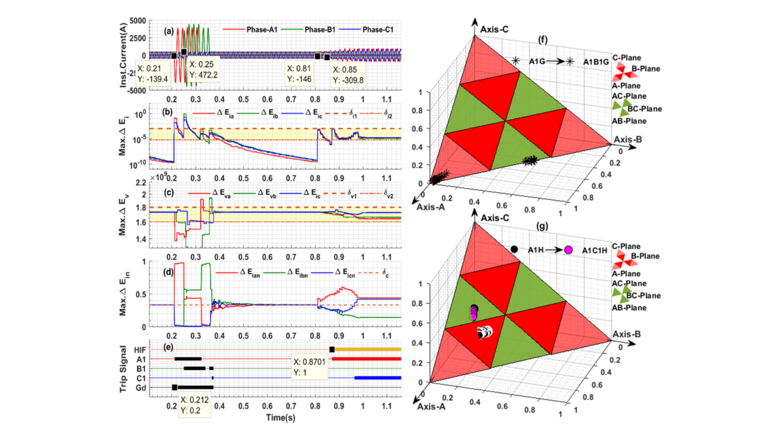
Figure 12 - Comparison of EVF (non-HIF) vs EVF-HIF fault: (a) Three-phase currents (b) Max. change in MWPE of current signal (c) Max. change in MWPE of voltage signal (d) Normalized values of MWPE of current signal (e) FD scheme output (f) Classification of EVF (g) Classification of EVF-HIF [10]
4. Fault location (FC) scheme for CCFs in the DCTL using an optimized ensemble of regression trees
In this section, an Ensemble of Regression Tree (ERT)-model based fault location scheme has been proposed using an ensemble of regression trees such as Bagged Regression Trees (BGRT) and Boosted Regression Trees (BSRT). This ensemble of regression tree modules has been trained with optimized Hyper-parameters such as minimum leaf size, leaning cycles and learning rate by using Bayesian optimization. Distinct datasets have been designed at wide-range of fault scenarios thereby applying an exclusive signal processing technique such as Discrete Wavelet Transform (DWT). The proposed scheme has been validated with real-time dataset which is generated on RSCAD/RTDS setup, cited in [11, 17]. The simulation results reveal the applicability of proposed ERT-model for fault location estimation and it gives a research insight to adopt the same in CSPT network.
4.1. Proposed ERT-model based fault location scheme for CCFs
The ERT-model works with CCFs typically from DCTL in different zones at different phases at the same time. Here this ERT model includes fault locator modules (BGRT-1, 2 and 3). With the help of these fault locator modules (BGRT-1, 2 and 3), the CCF location can be measured using only one end data of DCTL. Fig.13 shows the fault location scheme based on the ERT model. It contains of two segments, in the segment-I, training and validation of ERT-model is performed and, in the segment-II, an ERT-model test is performed. Regression tree-based ensemble methods such as BGRT and BSRT develops simple / standard tree-based techniques [12, 13].
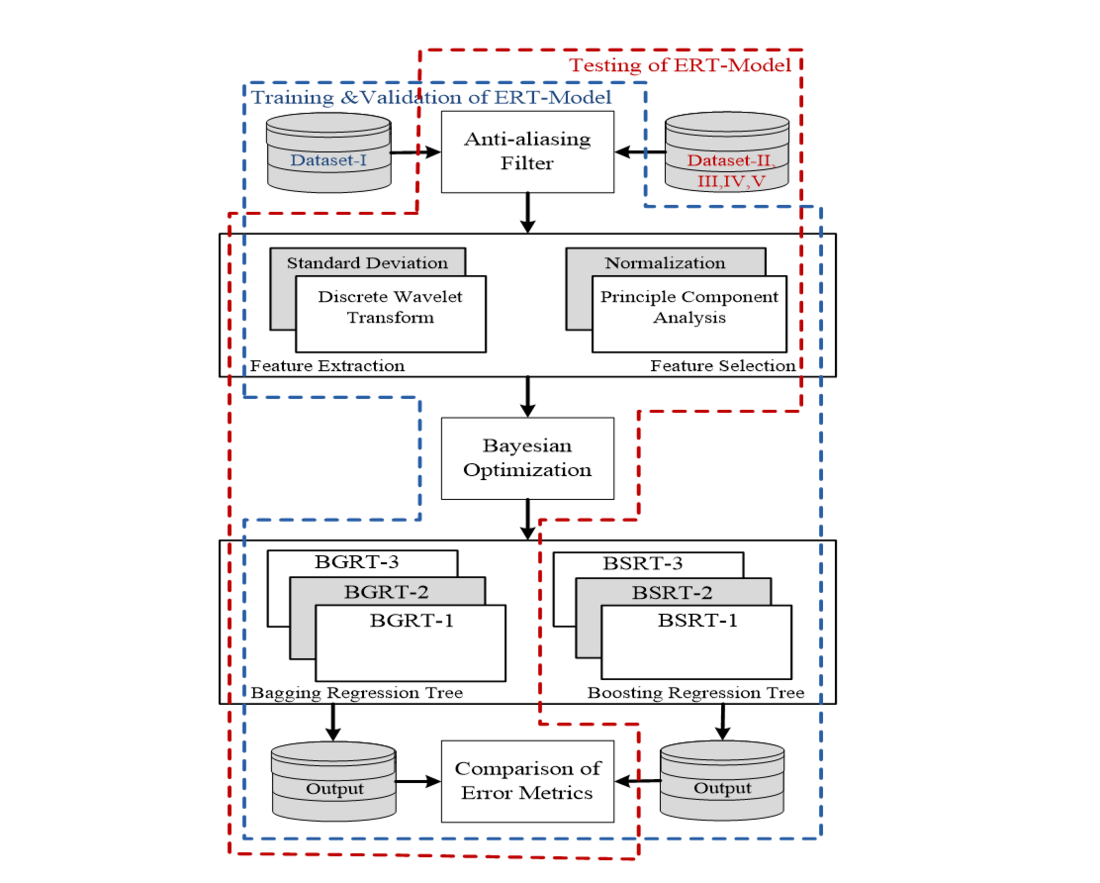
Figure 13 - Block diagram of proposed scheme for location of CCFs [11]
4.2. Design of an exclusive dataset to erudite fault locator modules
Special data sets are generated by mimicking fault circumstances across the DCTL of CSPT network in the MATLAB / Simulink software [11]. In addition, voltage & current signals are logged at 1.0 kHz frequency sample. It is very significant to excerpt the suitable topographies from the voltage/current signal in order to design special data sets for training / testing of fault locator modules since the efficiency of the ERT-model is subject to the learning capability of a ensemble of regression trees. Herein this proposed scheme an illustrative signal processing technique such as DWT has been used to extract relevant features. The significant features are extracted from three phase currents of circuit-I & II and three phase voltages of sending-end bus as well. Table 1 demonstrates variation of fault parameters to generate an exclusive dataset-I.
| Parameter | Training/ Testing |
|---|---|
Lf (km) | (1-197) in steps of 1 km |
| 0, 90 and 270 |
Rf ( | 0, 50 and 100 |
Ft : No. of Fault Cases | (A1G-B1G): 86436 |
Total No. of Fault Cases | 3 ˟ 86436= 259308 |
a. Principle Component Analysis (PCA)
A feature selection approach, PCA has been used to decrease computational burden by eliminating undesired topographies/features of input data set and it advances accurateness in fault location estimation during the training and testing. The PCA delivers perceptions into the freedom of choosing the significant feature as an input to the regression tree modules.
b. Bagged Regression Tree
BGRT is randomly creates multiple regression trees and before compiles their predictions. Every tree in the ensemble of bagging is enhanced by a different bootstrap simulation of the input data [12, 13]. The eccentric view in this representation is “outside the bag” of this tree [12, 14]. Therefore, grouping is just like as bootstrap aggregation for a group of regression trees. Each of the regression trees is usually extremely proportional / well proportioned. The ensemble of bagging method incorporates the effects of many regression trees, that minimizes the over-fitting problem and improves generalization.
c. Boosted Regression Tree
In this method combines different regression trees, which are repetitively designed by weighted/biased forms of the learning sample, with these weights adaptively attuned at each/every stage to give enhanced weight to the cases that were mis-classified in the previous step. Final predictions are achieved by measuring the results of a repetitive prediction. The BSRT is a tree-based ensemble method, such as a bagging, or a committee-based method that can advances the accurateness of regression methods. In contrast to bagging that uses a modest average to achieve a complete prediction, boosting uses a weighted measure of the results obtained by using a prediction method in a few input samples.
d. Optimization of the ERT modules
Choosing the right combination/ensemble method and the corresponding training constraints is a very challenging task. In addition, each method of integration has a inimitable feature that has both merits and demerits [11]. Therefore, it is necessary to select the appropriate ensemble method and the relevant training constraints (Hyper-parameter) such as minimum leaf size, number of learning cycles and learning rate. In this regard, Bayesian Optimization has been adopted to find optimum number of training constraints [15].
4.3. Training/validation of fault locator modules of ERT-Model
The fault locator modules of ERT-model are trained and tested extensively to evaluate the generalized performance of fault locator modules at the wide range of fault scenarios. In this regard a cross-validation method has been considered and further fault locator modules are trained/tested by performing various case studies using different combination of data sets for training and testing purpose correspondingly, such as case-1(90/10), case-2(80/20), case-3(70/30), case-4(60/40) and case-5(50/50). For example, a combination of (80/20) data set represents 80% of data is considered for training purpose and 20% of data set for testing purpose [11]. Generalized performance assessment of different BGRT modules for different combination of datasets with their corresponding outcomes/metrics such as Leaf size (Ls), Learning cycles (Lc), training time and different error metrics i.e., Mean Absolute Error (MAE), Mean Absolute Relative Error (MARE), Mean Square Error (MSE), Root Mean Square Error (RMSE).There are different methods to calculate fault location error as per IEEE Std. C37.114TM-2014 which is a revised version of IEEE Std. C37.114-2004 [16]. To understand a range of different error measurements using a specific fault location methodology for a particular power system network, a comprehensive error assessment has been exemplified in terms of different error metrics. These error metrics gives a kind of research insight to the protection/relaying engineers in a complete manner and also it is very useful to the line patrolling crew so that they can travel to an actual fault location to repair a faulty-equipment as quickly as.
4.4. Case studies with results and discussions
Extensive simulation has been carried out to generate an exclusive datasets (Dataset-II, III, IV,V) thereby varying different fault parameters (Lf =1-197km, f = 0°, 90°, 270° and Rf = 0Ω, 50Ω, 100Ω), sampling frequency ( fs =1kHz, 1.2kHz, 5kHz and 10kHz), data-window size (ws =1-cycle, 2-cycle and 3-cycle) and signal-to-noise ratio (SNR= 20dB,30dB and 40dB). Herein this work, the ERT-model has been tested for different CCFs to evaluate performance of different regression modules in fault location estimation in terms of error metrics. Fig.14 (a-c) shows performance of BGRT-1 module in terms of different error metricsfor fault1/fault2 at different fault parameters with Rf =0Ω, 50 Ω and 100 Ω and
f = 0°, 90°, 270° respectively. Fig.15(a-b) shows the performance of BGRT-1 module for variation in sampling frequency in case of fault1 (A1G) and fault2 (B1G) of a cross-country fault (A1G-B1G). From Fig.16 (a-b), the MARE is decreased linearly in case of fault1 and fault2 with respect to the variation in SNR. The comparative assessment has been done thereby comparing overall performance assessment of different ERT modules such as BGRT and BSRT which elaborates comparison of outcomes of training/testing of different fault locator modules. Fig.17 exemplifies the comparison of error metrics of BGRT-2 and BSRT-2 modules for a CCFs (A1G-B1C1G).
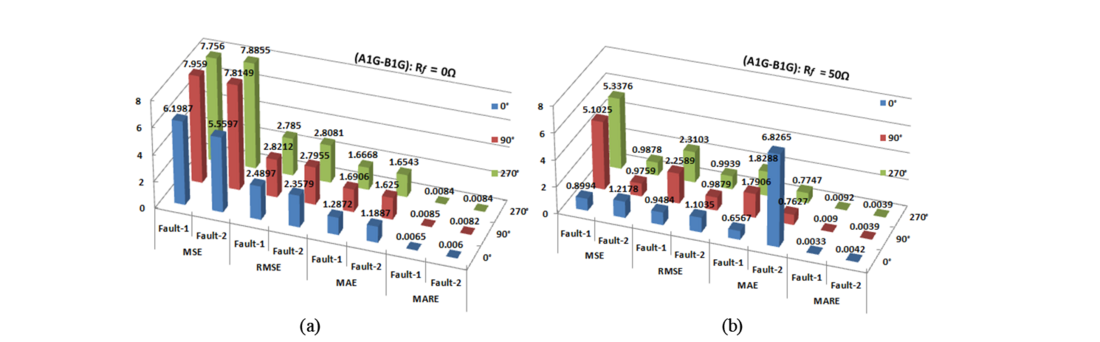
Figure 14 - Error metrics of fault locator module (BGRT-2) for CCFs at ϕ_f= 0°, 90°, 270°: (a) R_f= 0Ω, (b)R_f= 50Ω [11]
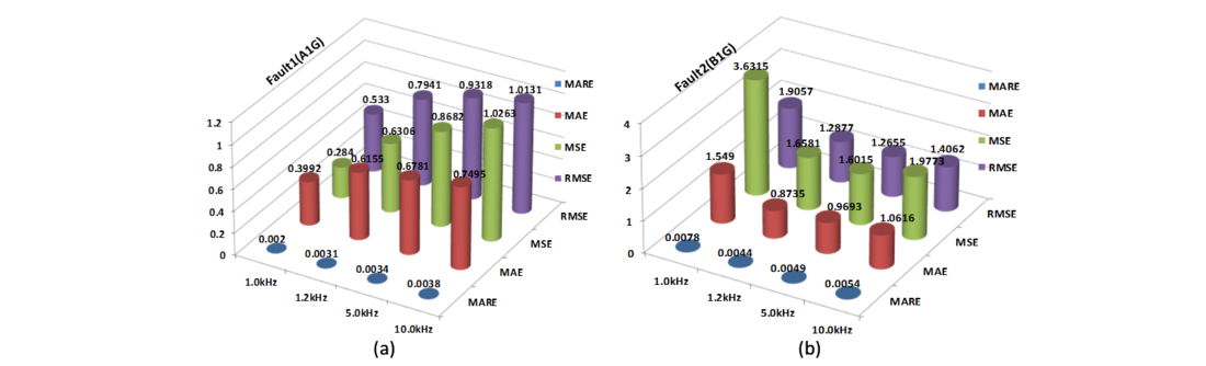
Figure 15 - Error metrics of fault locator module (BGRT-1) for CCFs with variation in sampling frequency (f_s): (a) Fault1(A1G) (b) Fault2(B1G) [11]
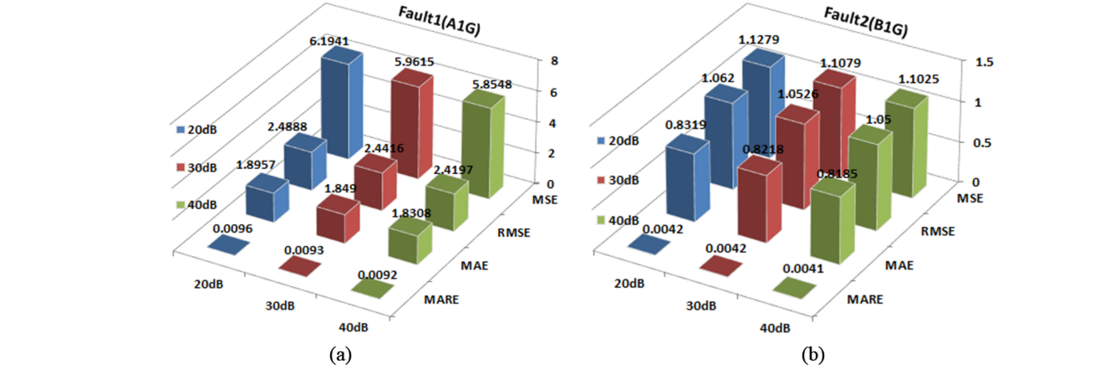
Figure 16 - Error metrics of fault locator module (BGRT-1) for CCFs with variation in SNR: (a) Fault1(A1G) (b) Fault2(B1G) [11]
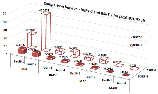
Figure 17 - Comparison of error metrics of BGRT-1 vs BSRT-1 for location of CCFs (A1G-B1G) [11]
Nevertheless, accurateness of the proposed scheme is represented by error metrics such as MAE, MARE, MSE and RMSE. The least error indicates exactness in the estimation of fault position. In view of this, from all the test cases, MAE is ranged between 0.0060 and 6.8265, MARE is ranged between 0.0020 and 0.0136, MSE is ranged between 0.00005 and 11.8430 and RMSE is ranged between 0.0037 and 3.4414. The proposed scheme has been validated with real-time dataset which is generated on RSCAD/RTDS setup to evaluate adaptability in practical power system network [11, 17].
5. Data-mining model for location of evolving faults (EVFs) using an optimized ERTs
In this section, a data-mining model based fault location scheme has proposed using BGRT and BSRT for EVFs. This ERT modules has been erudite with optimized training constraints (hyper-parameters) by using Bayesian optimization. Exclusive datasets have been designed by performing extensive simulation studies at wide-range of fault scenarios thereby applying an explanatory signal processing technique such as DWT. Further performance assessment has been carried out by comparing different error metrics like MAE, MARE, MSE and RMSE etc [16]. The outcomes of this fault location scheme explore the applicability of proposed data-mining model and it explores a research perception while adopting the same to practical CSPT network [18].
5.1. Proposed Data-Mining model for location of EVFs
This data-mining model includes three fault locator modules (BGRT-1, 2 and 3). These fault locator modules are designed for three atypical EVFs such as (A1G-B1G) fault, (A1G-B1C1G) fault and (A1B1G-C1G) fault which are the furthermost important of all EVF types. For example, EVFs(A1G-B1G) is a combination of two faults, fault1 (A1G) and fault2 (B1G) occurring at the same location at different fault inception time at different phases in the same transmission circuit-I. With the help of these fault locator modules (BGRT-1, 2 and 3), the location of EVFs has been done using only one terminal data of DCTL. Fig.18 shows the fault location scheme based on the data-mining model. It consists of two phases, in the first phase training and validation of the extraction model is performed and in the second phase the testing of a trained extraction model is carried out.
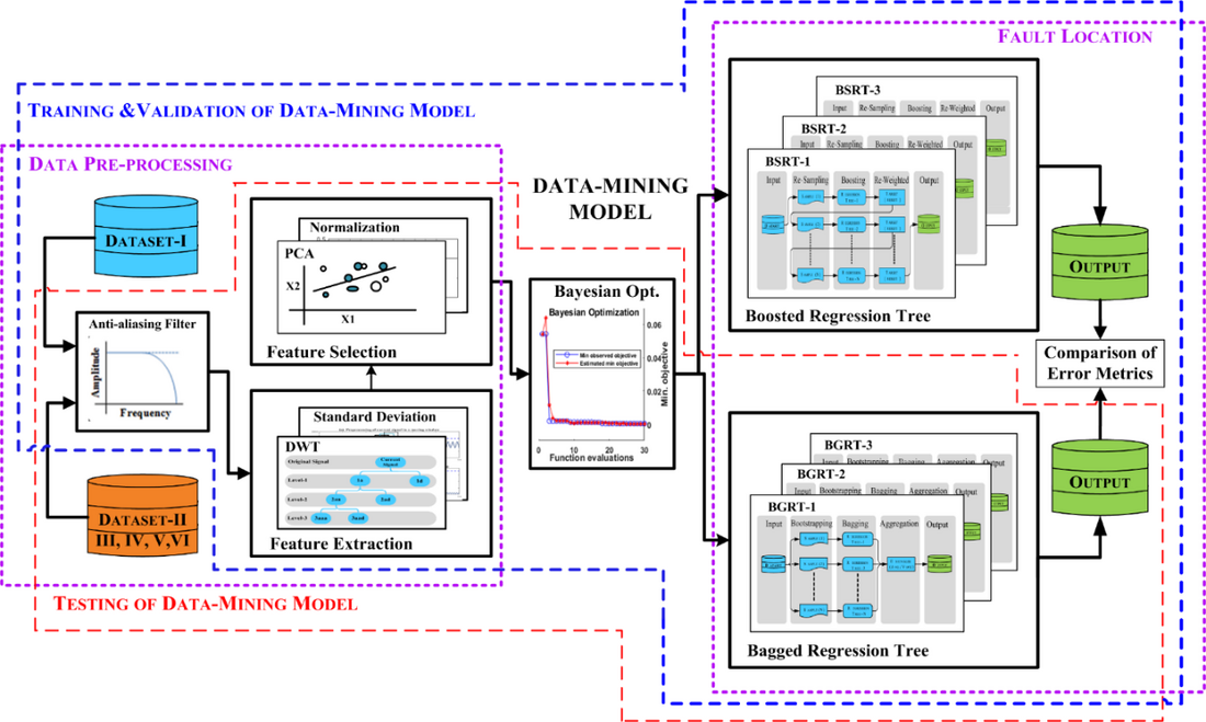
Figure 18 - Proposed data-mining model-based fault location scheme for EVFs [18]
5.2. Design of an exclusive dataset to erudite fault locator modules
In this proposed data-mining model, special data sets are generated by mimicking fault scenarios across the CSPT in the MATLAB / Simulink software. In addition, voltage and current signals are recorded in the 1.0 kHz frequency sample. It is very significant to excerpt the suitable features from the faulty signal to design specific data sets for training / testing of BGRT modules because the efficiency of the data simulation model be subject to the learning capabilities of the setbacks. Here the proposed system used a digital signal processing method such as DWT to extract the appropriate attributes. In the proposed scheme, a special data set is designed to train and evaluate the data-mining model to develop accurate fault detection modules (regression tree module) for EVFs as shown in Table 2.
Parameter | Training/ Testing |
|---|---|
Ft / No. of Fault Cases | (A1G-B1G) fault: 197 (Lf ) ˟ 3 ( |
Lf (km) | (1-197) in steps of 1 km |
| 0, 90 and 270 |
Rf ( | 0, 50 and 100 |
Ef (Fault Evolving Time in ms) | 10, 20, 40, 60, 80 and 100 |
Total No. of Fault Cases | 3(Ft ) ˟ 3 (Lf ) ˟ 3 ( |
a. Principle component Analysis (PCA)
A feature choosing method using PCA has employed to decrease computational intensity by eliminating undesired features and it progresses accurateness of fault locator modules in training/testing. This PCA offers perceptions into the freedom of the candidate feature which can be useful as input during training/testing of fault locator modules.
b. Bagged Regression Tree
BGRT is randomly creates multiple regression trees and before compiles their predictions. Every tree in the ensemble bagging is enhanced by a different bootstrap simulation of the input data [14, 18]. The eccentric view in this representation is “outside the bag” of this tree [13, 18]. Therefore, grouping is nothing but bootstrap aggregation for an ERTs. Each of the regression trees is usually extremely proportional / well proportioned. The ensemble of bagging method incorporates the effects of many regression trees, that minimizes the over-fitting problem and advances generalization.
c. Boosted Regression Tree
BSRT is a method of combining different regression trees, which are repetitively (iteratively) formed by weighted/biased forms of the learning sample, with these weights adaptively attuned at each/every stage to give enhanced weights to the cases that were mis-classified in the previous stage. Final predictions are achieved by measuring the results of a repetitive prediction. The BSRT is a tree-based ensemble method, such as a bagging, or a committee-based method that can enhances the efficacy of regression methods. Unlike bagging that uses a simple measurement of results to achieve a complete prediction, the boosting uses a moderate estimate of the results attained using the prediction method in a few input samples [18-20].
d. Optimization of the ERT modules
While there are some benefits by using a combination of regression trees over conventional regression trees, selecting the right ensemble method and the corresponding training constraints (Hyper parameter) is a very challenging task. In addition, each method of ensemble has an inimitable feature that has both advantages and disadvantages. For example, the process of assembling bags often creates deep trees, this leads to a time-consuming and memory-intensive process that provides slower predictions. With the exception of other hybridization methods that usually use very shallow trees, their construction requires little time or memory but in order to be effective, it requires more integrated members than tree-packed trees. Selecting a joint member size includes measurement speed and accuracy. Therefore, it is not always clear which method of ensemble is best. Therefore, it is necessary to select the suitable method of integration and the appropriate training constraints (Hyper-parameter parameter). In this regard, the Bayesian Optimization has been used to determine suitable hyper-parameters [15, 18].
5.3. Training/validation of regression tree modules of data-mining model
An exclusive data set has been designed to train and test the data-mining model for developing accurate fault locator modules for EVFs as shown in Table 2. Fig.18 demonstrates proposed fault location scheme based on data-mining model. It comprises of two stages, in the first stage training and validation of the data-mining model is carried out and in the second stage testing of the trained data-mining model has been done. The proposed data-mining model is trained and tested extensively to evaluate the generalized performance of fault locator modules at the wide range of fault scenarios. In this regard a cross-validation technique has been considered and further fault locator modules are trained/tested by performing various case studies using different combination of data sets for training/testing purpose correspondingly, such as case-1 (90/10), case-2 (80/20), case-3 (70/30), case-4 (60/40) and case-5 (50/50). For example, in the case-2 a combination of (80/20) data set represents 80% of data is considered for training purpose and 20% of data set for testing purpose. Generalized performance assessment of different BGRT modules for different combination of datasets with their corresponding outcomes/metrics such as Leaf size (Ls), Learning cycles (Lc), training time and different error metrics i.e., MAE, MARE, MSE, and RMSE. There are different methods to calculate fault location error as per IEEE Std C37.114TM-2014 which is a revised version of IEEE Std C37.114-2004 [16, 18]. To understand a range of different error measurements using a specific fault location methodology, for a particular power system network, a comprehensive error assessment has been exemplified in terms of different error metrics. These error metrics explores a kind of research insight to the protection/relaying engineers in a comprehensive manner and also it is very useful to the line patrolling crew so that they can travel to an actual fault location to repair a faulty-equipment as quickly as.
5.4. Case studies with results and discussion
It is very significant to evaluate the performance of proposed fault location scheme based on data-mining model, in this context an extensive simulation studies have been performed to design an exclusive datasets (Dataset-II, III, IV,V,VI) thereby varying different fault parameters (Lf =1-197km, f = 0°, 90°, 270°and Rf = 0Ω, 50Ω, 100Ω), fault evolving time (Ef = ½ , 1, 2, 3, 4, 5-cycle), sampling frequency (Fs =1kHz, 1.2kHz, 5kHz and 10kHz), data-window size (Ws =1-cycle, 2-cycle and 3-cycle) and signal-to-noise ratio (SNR= 20dB, 30dB and 40dB). Herein this section, the data-mining model has been tested for different EVFs to evaluate performance of different regression modules in fault location estimation in terms of error metrics. Fig.19 (a-c) illustrates the performance of BGRT-2 module in terms of different error metrics for fault1/fault2 at different fault parameters with Rf =0Ω, 50 Ω and 100 Ω and
f = 0°, 90°, 270° respectively. Fig.20 (a-b) shows the performance of BGRT-2 module for variation in sampling frequency in case of fault1(A1G) and fault2 (B1C1G) of an evolving fault (A1G-B1C1G). Fig.21(a-b) demonstrations the performance of BGRT-2 module for variation of SNR in case of fault1(A1G) and fault2 (B1C1G) of an evolving fault (A1G-B1C1G). The comparative assessment has been done thereby comparing overall performance assessment of different ensemble of regression tree modules such as Bagged Regression Tree (BGRT) and Boosted Regression Tree (BSRT) which elaborates comparison of outcomes of training/testing of different fault locator modules [18]. Fig.22 illustrates the comparison of outcomes of BGRT-2 versus BSRT-2. Furthermore, the accuracy of the proposed fault location scheme has been analyzed in terms of error metrics such as MAE, MARE, MSE and RMSE. The minimum error shows more accuracy in fault location estimation. In this context, considering all the test cases performed in the study, the range of MAE is between 0.0032 to 1.9641, MARE is between 0.0009 to 0.0240, MSE is between 0.00003 to 125.3311 and RSME is between 0.0037 to 11.1951. In the proposed fault location scheme bagged regression tree approach showing a minimum error which enhances the reliability of the power transmission system by reducing outage time. It is also worth to mention computer system configuration when dealing with machine learning techniques such as decision/regression tree algorithm, support vector machines, artificial neural network etc. since the CPU speed and its internal memory capacity plays an important role while pre-processing of raw data, training/testing as well. This research work has been carried out on Intel® Xeon® CPU E3-1225 v5 @ 3.30GHz processor with 16GB RAM 64-bit Windows 7 operating system.
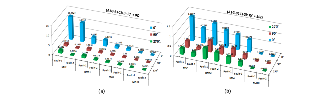
Figure 19 - Error metrics of fault locator module (BGRT-2) for EVFs: (a) R_f= 0Ω, ϕ_f= 0°, 90°, 270° (b) R_f= 50Ω, ϕ_f= 0°, 90°, 270° [18]
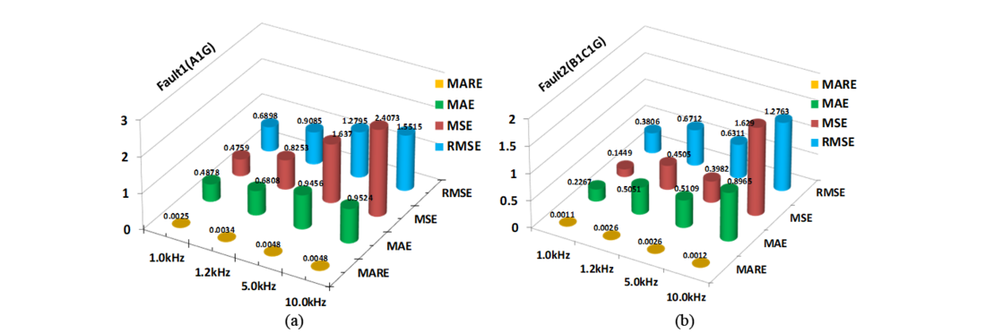
Figure 20 - Error metrics of fault locator module (BGRT-2) for EVFs (A1G-B1C1G) with variation in sampling frequency(f_s): (a) Fault1(A1G) (b) Faul2(B1C1G) [18]
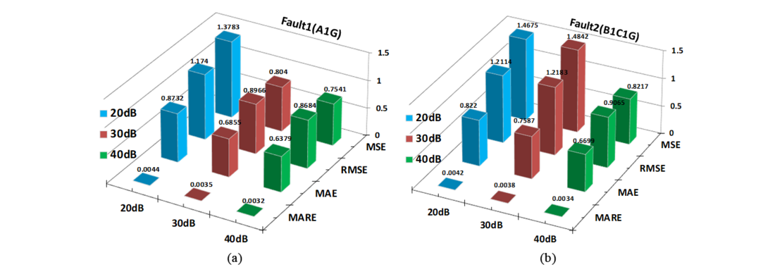
Figure 21 - Error metrics of fault locator module (BGRT-2) for EVFs (A1G-B1C1G) with variation in SNR: (a) Fault1(A1G) (b) Fault2(B1C1G) [18]
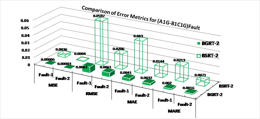
Figure 22 - Comparison of error metrics of BGRT-2 vs BSRT-2 for location of EVFs (A1G-B1C1G) [18]
6. Conclusions
In this Ph.D. thesis work, pattern recognition technique and advanced signal processing techniques-based protection schemes have been presented to mitigate the issues associated with the distance protection (Zone-1) on DTCL of CSPT network. Mainly, in this research work addressed three atypical fault scenarios which occurs frequently in large scale electric power transmission network, i.e., CSPT network. Several relaying algorithms have been designed/proposed using pattern recognition techniques and advanced signal processing techniques and the same have tested on CSPT network modelled/simulated in MATLAB/Simulink and RSCAD/RTDS setup. The specific contributions of this thesis work and their outcomes are considerable. Moreover, the proposed MODWT-based relaying scheme detects/classifies all types of CSFs during stable PS with a minimum 0.05 cycle to maximum 0.5-cycle time [5]. The performance was also evaluated for real-time field fault data recorded by DFR in a sub-station of an Indian power system utility and test results are appreciable. Another protection scheme has proposed based on MODWT for detection/classification of CCFs/EVFs has response time of ¼ -cycle to 1-cycle and also few fault cases are validated on a prototypical model of 180km power transmission line in the laboratory environment [8]. A Fault diagnosis scheme has been designed/proposed for detection/classification of CCFs/EVFs with HIF syndrome and testes for various switching events and presence of non-linear loads as well. Furthermore, the proposed scheme is demonstrated response time within 5-cycle [10]. A new fault location scheme based on ERT-model for CCFs has been designed/proposed. However, the accuracy of this scheme in fault location estimation has analyzed using error metrics. Thus, considering all the test cases performed, BGRT modules exhibits minimum error in estimation of fault location; the MAE is varying from 0.0060 to 6.8265, MARE is varying from 0.0020 to 0.0136, MSE is varying from 0.00005 to 11.8430 and RMSE is varying from 0.0037 to 3.4414 [11]. Another fault location method based on data-mining model has confirmed minimum error in fault location estimation for EVFs. Though, considering all the test cases performed by BGRT modules, the ranges of MAE is between 0.0032 to 1.9641, MARE is between 0.0009 to 0.0240, MSE is between 0.00003 to 125.3311 and RSME is between 0.0037 to 11.1951 [18]. In addition to the above stated relaying schemes, other pattern recognition methods such as ANN, Bagged Decision Tree and Fuzzy Logic has been adopted in designing new relaying scheme. Moreover, advanced signal processing techniques such as DCT, DWT, DWPT, MODWT and MODWPT have been used to extract exclusive attributes from the faulty signals to design novel relaying scheme. Hence the pattern recognition-based protection schemes for detection/classification/location of atypical fault scenarios have reported in this thesis work and overall outcomes of this research work is appreciable.
References
- Mohamed A. Ibrahim, “Disturbance analysis for power systems”, Wiley-IEEE, 2012, page 48-51.
- F. B. Costa, B. A. Souza, and N. S. D. Brito, “A wavelet-based algorithm to analyze oscillographic data with single and multiple disturbances”, IEEE PES General Meeting, Pittsburgh, USA, June 2008.
- F. B. Costa, B. A. Souza, and N. S. D. Brito, “Real-time detection of fault-induced transients in transmission lines”, IET Electronics Letters, pp. 753–755, May 2010.
- F. B. Costa, B.A.Souza and N.S.D.Brito, “Real-time classification of transmission line faults based on maximal overlap discrete wavelet transform”, Proc. of PES T&D 2012, 7-12 May 2012, Orlando, FL, USA.
- V.Ashok and Anamika Yadav, “A Real-Time Fault Detection and Classification Algorithm for Transmission Line Faults Based on MODWT during Power Swing”, International Transaction on Electrical Energy Systems Volume 30, Issue 1, January 2020.
- Fabio Massimo Gatta, Alberto Geri, Stefano Lauria and Marco Maccioni, “An equivalent Circuit for Evaluation of Cross-Country Fault Currents in Medium Voltage (MV) Distribution Networks”, Energies 2018, 11, 1929.
- Asia Codino, Fabio Massimo Gatta, Alberto Geri, Stefano Lauria, Marco Maccioni and Roberto Calone, “Detection of Cross-Country Faults in Medium Voltage Distribution Ring Lines”, AEIT International Conference 2017, Cagliari, Italy.
- V.Ashok, Anamika Yadav and Almoataz Y. Abdelaziz, “MODWT-Based Faults Detection and Classification Scheme for Cross-Country and Evolving Faults”, Electric Power Systems Research, Volume 175, October 2019.
- Denis Keuton Alves, Flavio B. Costa, Ricardo Lucio de Araujo Ribeiro, Cecilio Martins de Sousa Neto and Thiago de Oliveira Alves Rocha, “Real-Time Power Measurement Using the Maximal Overlap Discrete Wavelet-Packet Transform”, IEEE Trans. on Industrial Electronics, vol.64 No.4, April 2017, pp. 3177-3187
- V.Ashok and Anamika Yadav, “Fault Diagnosis Scheme for Cross-Country Faults with Emphasis on High-Impedance Fault Syndrome”, IEEE Systems Journal, Date of Publication: 25 May 2020, pp. 1-11.
- V.Ashok, Anamika Yadav, M Pazoki, Almoataz Y. Abdelaziz, “Fault Location Scheme for Cross-Country Faults in Dual-Circuit Line Using Optimized Regression Tree”, in Electric Power Components and Systems, 2020.
- V.Ashok, Anamika Yadav, C.C. Anthony, K.K. Yadav, Umakant Yadav, Chapter 18 – “A reliable decision-making algorithm for fault during power swing in 400kV double-circuit transmission line: a case study of Chhattisgarh state power system network”, Editor(s): Shady H.E. Abdel Aleem, Almoataz Youssef Abdelaziz, Ahmed F. Zobaa, Ramesh Bansal, Book title “Decision Making Applications in Modern Power Systems”, Academic Press, 2020, Pages 473-506.
- Breiman, L. Machine Learning (1996) 24: 123. doi: 10.1023/A:1018054314350
- R. Polikar, "Ensemble based systems in decision making," in IEEE Circuits and Systems Magazine, vol. 6, no. 3, pp. 21-45, Third Quarter 2006.
- Available online at https://towardsdatascience.com/an-introductory-example-of-bayesian-optimization-in-python-with-hyperopt-aae40fff4ff0.
- IEEE Guide for Determining Fault Location on AC Transmission and Distribution Lines, IEEE Std. C37.114-2014, Power System Relaying Committee, IEEE Power and Energy Soc. Public., Dec10, 2014, pp.1–59.
- V.Ashok and Anamika Yadav, “A Protection Scheme for Cross-Country Faults and Transforming Faults in Dual-Circuit Transmission Line using Real-Time Digital Simulator: A Case Study of Chhattisgarh State Transmission Utility” Iranian Journal of Science and Technology, Transaction of Electrical Engineering 43(4), 941-967, 2019.
- V.Ashok, Anamika Yadav, M Pazoki, Ragab El Sehiemy “Optimized Ensemble of Regression Trees-Based Location of Evolving Faults in Dual-Circuit Line”, accepted in Neural Computing and Applications, 2020.
- V.Ashok, Anamika Yadav and Almoataz Y.Abdelaziz and M Pazoki, Chapter-3, titled– “An Intelligent Scheme for Classification of Shunt Faults including Atypical Faults in Double-Circuit Transmission line”, text book titled, “Artificial Intelligence Applications in Electrical Transmission and Distribution Systems Protection”,22 Oct 2021
- V.Ashok and Anamika Yadav, “A Novel Decision Tree Algorithm for Fault Location Assessment in Dual-Circuit Transmission Line based on DCT-BDT Approach” Presented in 18th International conference on Intelligent Systems Design and Applications (ISDA-2018) on 6th to 8th Dec 2018 at VIT, Vellore (T.N).