Secondary arc extinction in AC/DC overhead lines
Authors
M. RATAJCZYK, D. HART, A. BERTINATO – SuperGrid Institute, France
M. BELEY, C. DELGADO DÍAZ DE LEÓN, G. YIN, L. ZHENG, E. SELLIN – INSA Lyon, France
A. XEMARD – EDF, France

Summary
This paper focuses on a specific issue related to hybrid AC / DC overhead transmission lines: the extinction of the secondary arc current of a faulted DC pole. A pole-to-ground fault leads to an opening of breakers to interrupt the short-circuit current. If the line is long, a small AC current (a few 10ths Amps) keeps on circulating in the fault due to the inductive and capacitive coupling between the AC circuit and the faulted pole. This current is named the secondary arc current. It may disappear after some time. However, if the pole is reclosed before its extinction, the fault starts again. This is studied through the paper with a sensitivity analysis of different secondary arc parameters. Calculations conducted with an Electromagnetic Transient Program show that the transposition of the AC circuit can significantly reduce the secondary arc current and then the dead time following a DC fault.
Keywords
Hybrid AC/DC transmission line - EMTP-like program - Secondary arc - Dead time - DC protection - DC SPAR1. Introduction
Increasing electricity production and consumption, and the presence of renewable energy sources lead to the need for higher transmission capacities and a more flexible electrical grid. To meet this demand, an effective way to strengthen the grid involves transforming some AC overhead transmission lines into DC overhead lines. Then the idea of hybrid AC/DC transmission lines came up: AC and DC systems on the same tower [1][2]. The paper is devoted to the study of a specific technical issue related to these hybrid AC / DC lines: the extinction of the AC-side induced Secondary Arc Current (SAC) of a faulted DC pole. In case of a protection strategy based on Single Pole Auto-Reclosing (DC SPAR), a single-pole DC fault along a hybrid line leads to the opening of the breakers of the faulted pole to interrupt the DC short current. DC SPAR significantly strains the DC breakers and if the reclosing is not successful, they absorb a significant amount of energy [3]. If the line is sufficiently long, after the breakers’ opening, a small AC current, namely the SAC, keeps on circulating in the fault due to the electromagnetic coupling between the AC phase conductors and the pole. If the pole is reclosed before the extinction of the SAC, the fault starts again because the electrical channel engendered by the initial fault is still a path for the DC short-circuit current. On the other hand, a late reclosing may lead to stability issues.
The goal of this paper is to identify the factors which have a significant influence on the amplitude of the SAC in steady-state conditions (transient is not considered) and to study the efficiency of several solutions aimed at reducing its amplitude. The article is based on EMTP version 4.0.1. simulation performed in the frequency domain [5].
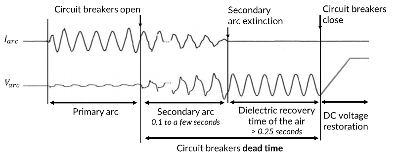
Figure 1 - Illustration of the arc current and voltage during the auto-reclosing procedure. Figure based on paper [4]
The outline of this paper is as follows: section 2 clarifies the conventional background knowledge of AC/DC hybrid lines, regarding electromagnetic coupling and the existing methods of extinction of secondary arc. Section 3 describes the line configuration that was selected for the studies, then the EMTP simulation model is presented in section 4. The following section is devoted to a parametric study of the SAC and to the analysis of solutions to reduce the time when the circuit breakers are opened which is called dead time. Conclusions are summarized in section 6.
2. Theoretical background and secondary arc extinction fundamental
This section recalls fundamental notions regarding the electromagnetic coupling between overhead conductors, and then the origin and extinction of the SAC. It ends with a presentation of solutions to reduce the duration of the SAC on AC lines.
2.1. The coupling between conductors
Two main types of coupling exist between the conductors of an overhead line [6]:
- Electrical coupling results from the electric field and is modelled by capacitances between conductors;
- Magnetic coupling is related to the magnetic field and is represented by mutual inductances.
This coupling induces an AC oscillation on DC pole current. Based on this assertion Figure 2 represents the coupling between the faulted pole and the surrounding conductors of a hybrid AC/DC line: capacitances model the electrostatic coupling, the voltage source “MA, MB, MC” models the magnetic coupling and the inductance “L” is the self-inductance of the pole. Lineic resistance is neglected in the figure.

Figure 2 - Capacitive and magnetic coupling between a pole and other conductors on a hybrid line [7]
In [8] the author shows how inductive coupling can be neglected when evaluating SAC for the design of hybrid overhead lines whilst capacitive coupling is predominant in normal operating conditions. Therefore, it is possible to simplify the representation by considering only the capacitances to obtain orders of magnitude of induced currents and voltages.
2.2. Arc Extinction
To avoid stability issues [9] or un-wanted actions by the protection relays [10], the order of value of the dead time on a DC line must be shorter than 1s, as illustrated by the South-West Link project in Sweden [11]. For a successful reclosing, the dead time must be longer than the extinction time of the secondary arc. Authors in paper [4], which deals with single-phase auto-reclosing in AC EHV systems, mention that short-circuit current preceding SAC and fault location have a strong influence on secondary arc extinction time. Their increase leads to a decrease in its duration. The recovery-voltage during arc-extinction is also an important parameter [12] and it also depends on the short-circuit current and on the characteristics of the secondary arc (high recovery voltage may lead to secondary arc reignition). Therefore, it is difficult to directly take it into account in practical studies. Moreover, according to [4], SAC which follows a high short-circuit fault, may exhibit severe transient recovery voltage (TRV). In addition, the external conditions around the arc-channel like the presence of ionized air, wind, thermal buoyancy, and electrodynamic forces have a strong influence on the secondary arc behavior and make its precise modelling a complicated matter [13]. Some authors proposed to model the secondary arc based on the Mayr equation and simulate the interaction of the secondary arc with the transmission system with an EMTP-like program. Their aim was to conduct parameter studies and to determine the instant when the secondary arc extinguishes in order to guess the worst case arcing time [13][14]. Based on the considerations regarding secondary arc behavior stated previously, it has been decided to apply in this study the conservative approach proposed by [4]. This paper, which presents an extensive set of lab-tests conducted to characterize the secondary arc current proposes to distinguish 2 sets of extinction phenomena:
- Type a – instantaneous break-off; a succession of breakdowns occurs until final extinction. In that case, the arc is interrupted in less than 0.15ms;
- Type b – steady-state extinction. The arc current decreases progressively until final extinction.
[4] suggests to disregard type a extinctions considering that they occur fast and are not problematic for fast reclosing, and to concentrate on type b extinctions for which an approach based on Equation 1 below is established. This equation relates the minimum dead time Tdead to consider and the peak amplitude of the SAC Is.
(1)
This equation has been empirically derived from field measurements and laboratory tests with AC overhead lines up to 700 kV. Its application to the extinction of the SAC following a DC fault on a hybrid AC/DC line, is a hypothesis made in this paper.
The forthcoming subsections present the methods to reduce the SAC following an AC fault on AC lines. Their applicability to hybrid AC/DC lines is considered in subsections 2.2.1 to 2.2.4 and relevant potential solutions were simulated in 5.2.
2.2.1. The effect of phase transposition on coupling reduction
Phase transposition [15] is a usual practice in AC systems and is recommended for EHV lines longer than 100 km [16]. It consists of a physical rotation of the conductors on the towers (Figure 3). It is performed in a way that the average mutual impedances (respectively admittances) become equal in the impedance (respectively admittance) matrices [15]. The transposition sequence refers to the direction of the rotation of the conductors when the transposition happens. The phase sequence indicates how the phases are positioned regarding the others (A-B-C or A-C-B). Appendix 7.5 provides a further understanding of these two parameters.
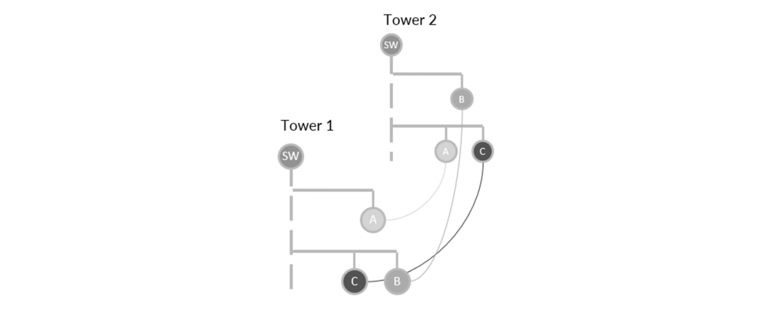
Figure 3 - Example of transposition configuration: phase sequence is clockwise and transposition sequence counter-clockwise
[17] and [4] present two transposition methods for double circuit AC transmission lines, with different costs and effectiveness. According to an example studied in [4] of a 700kV and 300km double circuit AC line, the most common line transposition type can reduces the SAC in AC of 30% and thus the dead time of 24%. For hybrid AC/DC transmission lines, the same considerations can be drawn. With the transposition, the three fields generated by the AC phases compensate and the overall coupling with the DC poles is therefore reduced [17].
2.2.2. Fast-earthing: High-Speed Earthing Switches (HSES)
HSES are installed at each end of lines to ground the faulted conductor after the opening of circuit breakers, as shown in Figure 4. Coordination of HSES and DCCBs is necessary in this case, the opening of the HSES needs to be precluded before the opening of DCCBs. This solution allows at the same time to facilitate the thermal extinction by reducing the SAC and the risk of dielectric breakdown by reducing the recovery voltage [18][12]. The secondary arc will be short-circuited during the dead time. It reduces the TRV, so it reduces the risk of arc reignition and increases the probability of a successful arc extinction [12]. TRV concern is out of the scope of this study. When the two HSES are closed, an electromagnetically induced current is created in each of the two loops formed by the secondary arc and the two HSES. The two currents flow in opposite directions and compensate each other (Figure 4). Thus, the magnetic component of the SAC is greatly reduced [19].
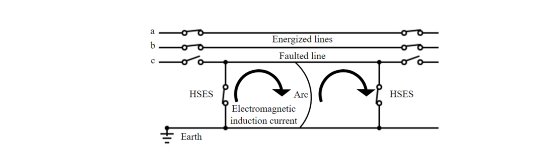
Figure 4 - Induced current in HSES and secondary arc [19]
Also, with the earthing of the faulted line, the line voltage collapses to an insufficient value to sustain the secondary arc, which thus extinguishes faster.
A delay between the opening/closure of circuit breakers and the opening/closure of the HSES is required to avoid any risk of station short-circuit. It is also possible to use a single HSES at one end of the line. All the current will flow in the HSES and the secondary arc, and consequently, the extinction will take more time.
2.2.3. Four-legged shunt reactor
Three shunt reactors (Ls in Figure 5) are usually installed between AC phases in a star configuration to compensate the reactive power supplied by the line. Shunt reactors are essential for long high voltage lines [20]. A degree of reactive power compensation of 70 to 80 % is a common practice [21].
The four-legged shunt reactors consist of adding a fourth reactance (Ln) between the neutral point and the ground, named the neutral reactor, as shown in Figure 5. The aim is to eliminate the capacitive coupling between the remaining sound phases and the faulted phase [22]. This creates an LC resonant circuit, in parallel between the phases, and it injects inductive current into the faulted phase, with opposite polarity compared to the capacitive current [21]. An analytical expression to size the neutral reactor based on the line specifications is provided in [21]. The estimation of the optimum shunt reactance value needs to consider all the possible fault locations along the line.
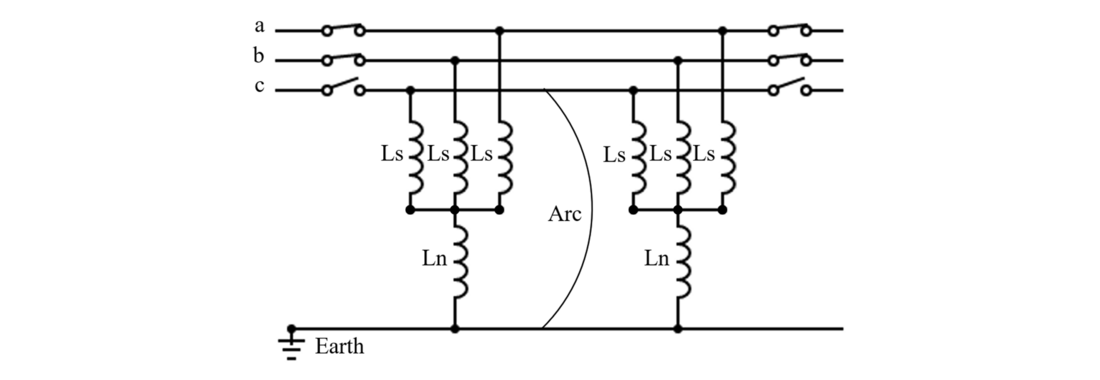
Figure 5 - Four-legged shunt reactors scheme
It is not possible to add shunt reactors on DC poles. But the influence of the four-legged shunt reactors installed on the AC circuit on the secondary arc is studied in this article.
2.2.4. By-pass capacitors
A shunt capacitor across the line breaker could be another solution. In normal operating conditions, the closed capacitors are shorted by the line breakers. When a fault occurs, the circuit breakers open and the secondary arc current is conducted into the capacitors during the dead time. According to [4], this circuit has a similar effect to that of four-legged shunt reactors. With appropriately dimensioned capacitors, the capacitive coupling can be compensated. It is also possible to introduce a single capacitor at one end of the line.
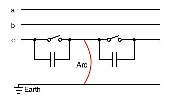
Figure 6 - By-pass capacitors
For notice, this method is only effective for single phase-to-ground faults [23]. It remains costly, due to the capacitor banks [4]. Besides, they need insulation coordination adapted to HVDC. So far, there is no known evidence against the adaptation of this solution for extinguishing the secondary arc on the DC pole of a hybrid line, but it has not been considered in this study.
3. Description of the considered configuration
This study is based on an existing overhead hybrid AC/DC high voltage line [24]. The 300 km line is 400 kV RMS at 50 Hz for AC and ±400 kV for DC systems, which is a bipolar configuration with a dedicated metallic return. The conductors used are ACSR (Aluminium Conductor Steel Reinforced) 265/35 and they are bundled with 4 sub-conductors and 60 cm spacers. The tower configuration is described in Figure 7 below. Further conductor data can be found in appendix 7.1.
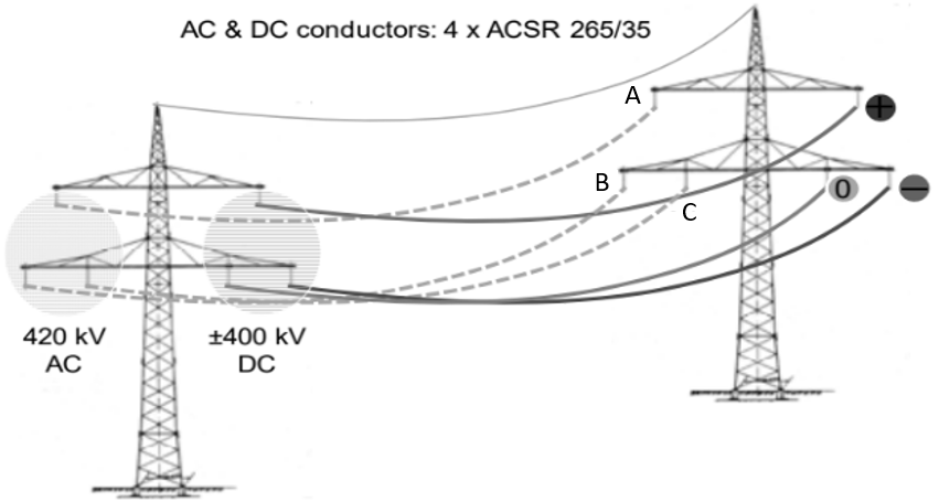
Figure 7 - Tower configuration [24]
4. Modelling of the system
The chosen simulation model is an exact-Pi multiphase representation of the line from its endpoints. Calculations are conducted in the frequency domain. On both ends of the AC line, a voltage source and series impedance of 19.5 Ω are added to represent the network that lies upstream and downstream of the line. Their value is calculated according to the IEC 60909 standard [25] using short-circuit current maximum values (see calculation in appendix 7.2). Load flow calculation is performed to conduct the simulations with AC lines (when healthy) current of 1 kA (RMS). The AC system is not compensated.
Each simulation or calculation is based on the same scenario: a pole-to-ground fault (primary arc) appears on one of the DC poles, and DC circuit breakers open only the faulted pole at both ends. The converters at both ends of the healthy pole are represented by grounding resistances of 1 Ω as proposed in [26] . The faulted pole is open-circuited at both ends. To consider the worst-case scenario, the fault is represented by a connection between the faulted pole and the ground via a resistance of 10 Ω, corresponding to the arc resistance and the grounding resistance of the faulted tower in parallel with the grounding resistance of the neighbouring towers. The metallic return (MR, solidly grounded on one end and grounded through a surge arrester on the other end) and the sky wire (SW, regularly earthed through 20 Ω resistances representing the ground and the tower resistance) are excluded from the simulations except if it is specified otherwise (see 5.1.4 for its configuration).
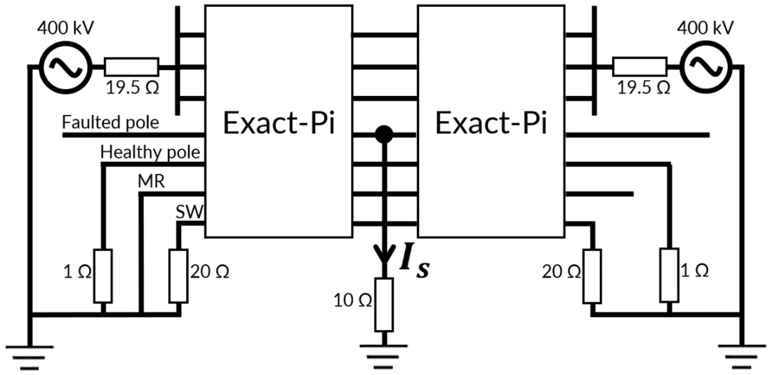
Figure 8 - Simulation scheme
5. Results
First, a parametric study is conducted to understand which factors influence the secondary arc extinction time and evaluate their impact. Then the retained solutions to reduce the dead time are investigated.
As explained in paragraph 2.2, an approximation of the required dead time can be made out of the arc current magnitude Is. The minimum significant dead time variation can be considered to be 50 ms. It corresponds to 5% of the maximum dead time according to the order of value proposed in section 2.2. This corresponds to a SAC variation of 2 A according to Equation 1. Therefore, throughout the whole study, a non-neglectable impact of the SAC on the dead time will be illustrated by a variation of more than 2A. To analyse the following results, an expression of the SAC was calculated (see details in appendix 7.4) :
(2)
E being the peak phase to ground voltage magnitude, a the cube root of unity, Rs the fault resistance, the susceptance between the faulted pole and a phase,
the susceptance between the faulted pole and the ground.
5.1. Parametric study
The SAC of the reference scheme built for the parametric study (see appendix 7.3) is 24.5 A (peak). This value was used as a reference to calculate the percentages in section 5.1, to visualize the variations cause by parameters and between parameters. The influence of the metallic return on the SAC was not studied in the parametric study.
5.1.1. Number of conductors per bundle
The number of conductors per bundle was changed from 1 to 6, leading to a total variation of the SAC of 24.5 A (100%).
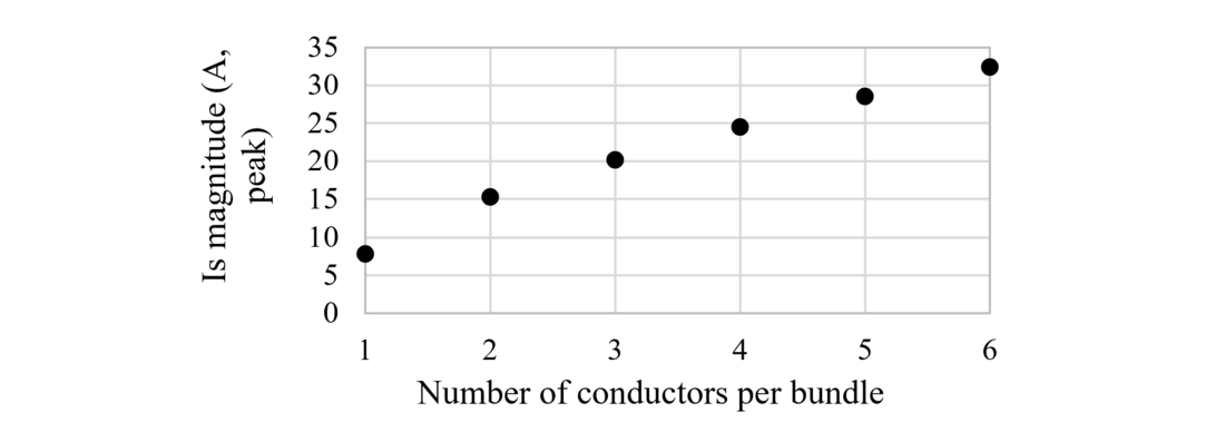
Figure 9 - Influence of the number of conductors per bundle on the SAC
Figure 9 confirms that the more conductors per bundle, the higher the SAC magnitude. This could be explained by the fact that the equivalent conductor total surface is increased, which could increase the electrostatic coupling.
5.1.2. Fault resistance
The study was conducted with values between 10 Ω (base-case scenario) to 2000 Ω, leading to variations of the SAC of 14.4 A (58.6%) according to simulations and 12.3 A (51.1%) according to analytical calculations (Equation 4).
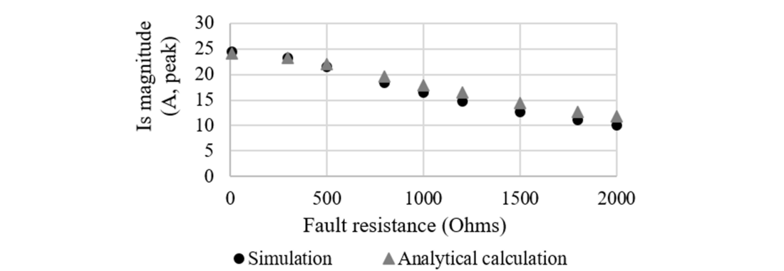
Figure 10 - Influence of the fault resistance on the SAC
Figure 10 confirms that the higher the fault resistance, the lower the SAC. If small resistances are considered, the SAC does not change much. In the paper, a conservative and more realistic value of 10 Ω was considered.
5.1.3. Line length
The total line length was changed between 200 and 800 km leading to a variation of the SAC of 61.1 A (250 %) according to simulation and 48 A (200%) according to analytical calculations (Equation 4). The same current and voltage were kept along the AC lines (400 kV RMS, 1 kA RMS). The fault location was kept at 25% of the line length from the beginning of the line.
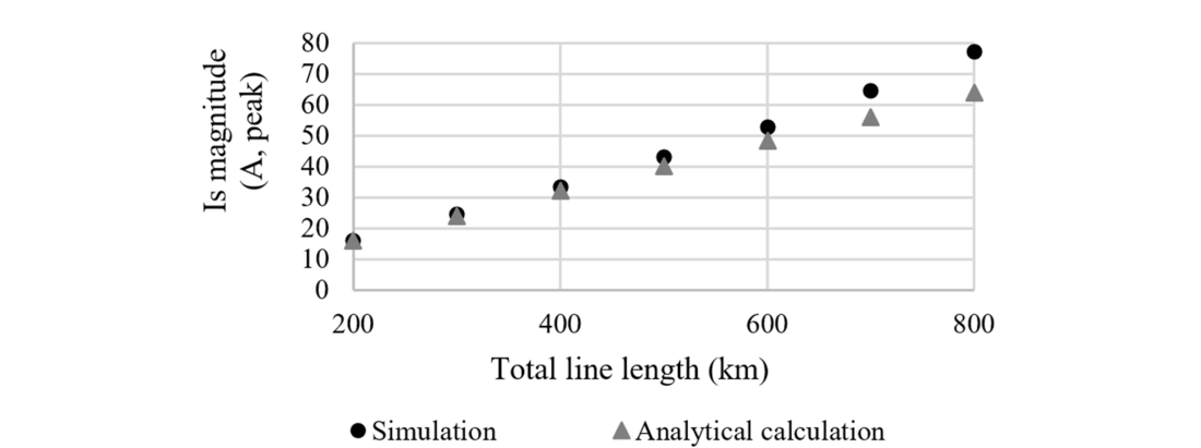
Figure 11 - Influence of the line length on the SAC
Capacitances being distributed along the line, means that the longer the line, the stronger the coupling and the higher the SAC magnitude. Lines longer than 400 km are almost always transposed, which would change the values of the average susceptances between the conductors and Figure 11 would not be relevant anymore. The right part of the graph thus represents a line configuration that would not exist in real life.
5.1.4. Sky wire
The simulated sky wire is earthed through 20 Ω resistances every 400 m for 1,6 km at each side of the fault location, and every 50 km elsewhere. The line is therefore 3.2 km longer than 300 km, but this issue has a negligible effect on the results.
| Sky wire | None | With |
|---|---|---|
Is magnitude (A, peak) | 24.5 | 20.1 |
Magnitude difference to ref in % | 0% | -17.9% |
According to Table 1, the sky wire seems to have a shielding effect that reduces the SAC by almost 18%. From an electrostatic point of view, the sky wire can be considered at zero volts. This means that the denominator of Equation 4 is increased (see appendix 7.4.2), which explains that the SAC is reduced. From a magnetic point of view, AC current is induced in the sky wire by the magnetic field created by the three AC phases. The induced current flowing in the sky wire will then create an induced magnetic field, which will, according to Lenz’s law, fight the variations of the magnetic field of the three AC phases. As a result, the total magnetic field is reduced, and its contribution to the SAC too.
5.1.5. DC pole positions
All six combinations of DC pole positions on the tower were simulated leading to a total variation of the SAC of 13.8 A (56.5%). Pole positions were named P1, P2 and P3 as shown in Figure 12.

Figure 12 - Poles position names on the tower
The presence of the sky wire and the metallic return impacts the influence of the pole positions on the SAC. Simulations were conducted with them included. In Table 2, the metallic return is located in the last available position (P1, P2 or P3).

Table 2 - SAC magnitude (A, peak) and difference to ref in % for different poles' positions
According to Table 2, the SAC magnitude seems to depend on the faulted pole but not on the healthy pole position as can be seen through the colours of Table 2. The best position is when the faulted conductor is the furthest from the AC system (P2). But whether the faulted pole is on P1 or P3 does not change the value of the current. The DC pole positions on the tower influence many other important issues such as the emission of ions by corona discharges which in turn enhance the electric field and produce ion current at the ground level [27]. It is therefore important, when there is no transposition, to keep the metallic return in the position P3, and the poles in P1 and P2, allowing the lowest SAC according to Table 2.
5.1.6. Fault location and AC current
he influence of the fault location and the AC current magnitude on the SAC were analysed together, a similar approach was used by authors in [26]. One set of simulations was conducted without AC current while keeping the nominal voltage, in order to evaluate the capacitive part of the SAC (fully black points in Figure 13). It is important to note that this configuration is not a usual operating condition and not in the scope of DC SPAR considered in this paper. According to Figure 13, the magnitude of the capacitive current is higher than the SAC created with both capacitive and inductive coupling. This suggests that there is compensation between the capacitive and the inductive parts of the SAC. Also, the capacitive secondary arc current only varies by 1.1 A (4.6%), which seems to confirm that the fault location has a negligible impact on the capacitive current, as the modelling suggested.
The fault location is responsible for variations from 0.7 A (3%) to 1.8 A (7.2%) depending on the AC current magnitude. The AC current magnitude is responsible for variations of 1.3 A (5.5%) to 2.4 A (9.6%) depending on the fault location. Both factors seem to have a very small impact on the SAC as shown in Figure 13.
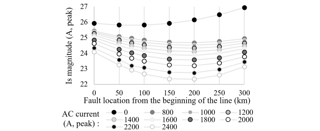
Figure 13 - Influence of the fault location and the AC current magnitude on the SAC
Some trends can be noticed:
- The higher the AC current, the lower the SAC.
- The higher the AC current, the bigger the variations on the SAC magnitude with the fault location.
- The current magnitude is higher on both ends of the line, and minimum in the middle.
Since the capacitive current is considered constant, the variations of the SAC observed are then due to the inductive current, which is related to the magnetic field created by the AC current in the phases. The higher the AC current, the higher the electromagnetic coupling, the higher the inductive SAC, the more the capacitive SAC is compensated by the inductive SAC and the lower the SAC.
In the literature ([26] and [4] for the same phenomenon in AC), the SAC trend with the fault location (minimum on both ends and maximum in the middle) is explained with the inductive current. The magnetic field created by the AC currents is orientated and so is the induced electromotive forces along the faulted pole. Consequently, the inductive current always flows in the same direction on the faulted pole. Therefore, the inductive currents from both sides of the fault loop in the opposite direction into the arc and compensate each other. It is the same phenomenon exploited by the HSES (see Figure 4), but on a smaller scale, because the inductive current loops through the capacitive coupling to the earth, and not through switches like in the case of HSES. The inductive SAC would then be highest for a fault on a line end and lowest in the middle. The angle between the inductive and capacitive currents could explain that the curves in Figure 13 have a minimum in the middle and not a maximum.
5.1.7. Line transposition
Two transposition cases were studied: when only the AC system is transposed and when both AC and DC systems are transposed (see Figure 14). The line was transposed five times (the line model was divided into six sections of 50 km). According to Table 3, the impact of both AC and AC/DC line transposition is similar: it reduces the SAC magnitude by up to 97%.
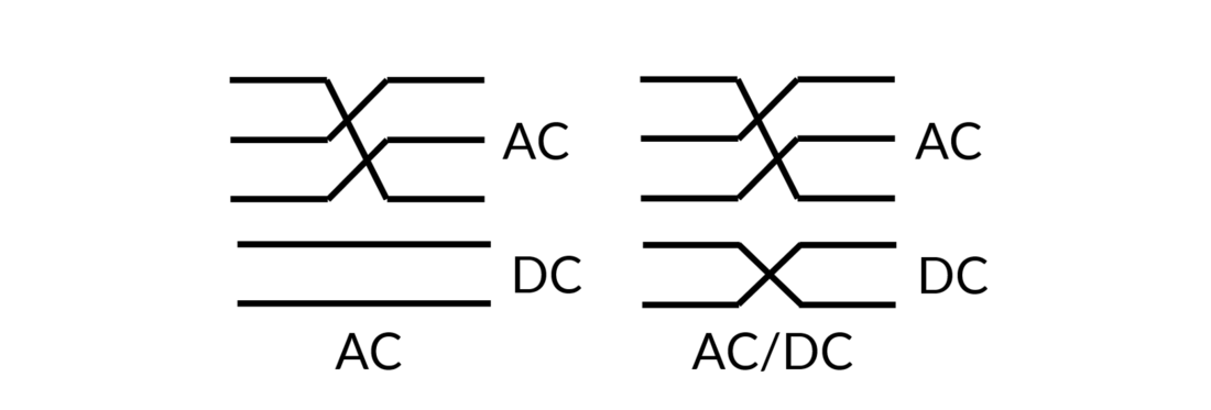
Figure 14 - Hybrid line transposition
| Transposition | None (ref) | AC | AC/DC |
|---|---|---|---|
Is magnitude (A, peak) | 24.5 | 0.72 | 0.85 |
Magnitude difference to ref in % | 0% | -97% | -96.5% |
By transposing the AC lines, the electric and magnetic fields are compensated along the line (see part 2.2). These results do not change if the DC line is also transposed, which enables a reduction of the influence of the DC lines on the AC lines and provides flexibility to engineers during the design phase of upgraded hybrid AC/DC lines.
5.1.8. Summary of factors’ influence
Figure 15 below summarize the results of the influence of factors investigated through section 5.1 through the magnitude difference to the reference case in percentage.
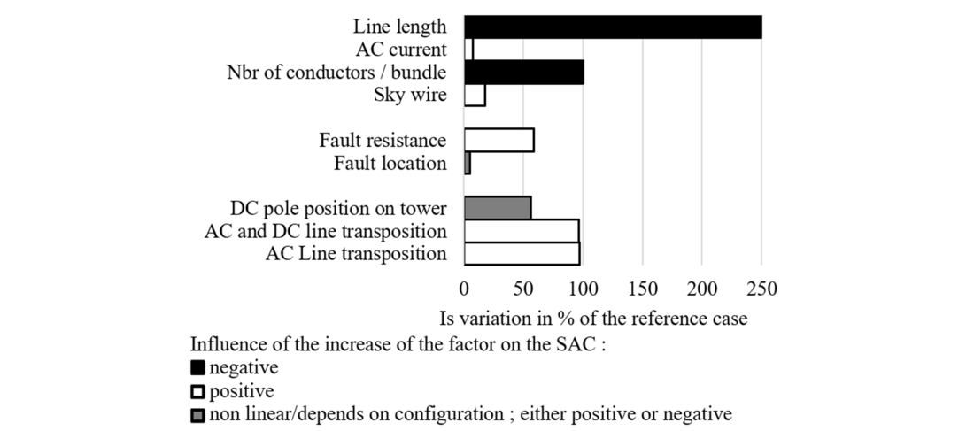
Figure 15 - Comparison of influencing factors on the SACs
In the case of upgrading a double circuit AC line to a hybrid line, some of the factors cannot be changed. According to Figure 15, line transposition could be an efficient solution to reduce the SAC. It will therefore be further studied in the next section through a new reference scheme. The contextual features (see appendix 7.3) will be set to their real values (see section 3) and parameters that cannot be controlled will be set to their worst-case scenario. The two best positions for DC poles on the tower are P2 and P1. As this study handles faults on both positive and negative poles, the chosen configuration to investigate solutions is to keep the healthy pole in P2 and the faulted one in P1. With this new reference scheme and SAC magnitude of 19.2A peak, some ideas of possible solutions to reduce the dead time were simulated. This value was used as a new reference to calculate the percentages in section 5.2, to visualize the variations due to and between different solutions. These results are presented in the next sections.
5.2. Investigation of solutions to reduce the dead time
This section presents results of an investigation of several potential solutions that could be applied to reduce the dead time.
5.2.1. Line transposition
5.2.1.1. General Study
Simulations were conducted by taking two parameters into account: the conductor and the transposition sequence (see appendix 7.5). Again, all transposition simulation schemes were built with 6 sections of 50 km, meaning 5 transpositions along the line. The metallic return (MR) is always taken into account, but it is not always included in the transposition.
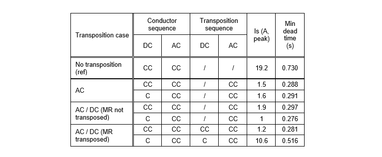
Table 4 - Line transposition simulations, fault located at the beginning of the line (CC : counter-clockwise ; C : clockwise)
AC line transposition and AC/DC line transposition with untransposed metallic return still seem to be equally efficient to reduce the SAC with a reduction to 1.5 A (92.2%) on average. But the transposition case of AC/DC line transposition with transposed metallic return has surprising results. The SAC varies from 1.2 A to 10.6 A (meaning a variation of dead time of 235 ms) depending on the pole and transposition sequence (two last rows of Table 4). To better understand the reason for this variation, this transposition case was studied more in depth, first by varying the fault location along the line (see Figure 16 below). It showed that the aforementioned variation remains all along the line. Then the conductor and transposition sequence were studied for a fault location of 75 km from the beginning of the line.
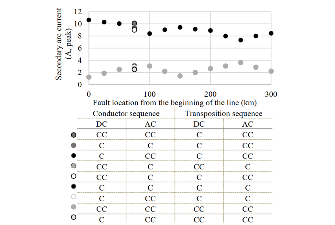
Figure 16 - AC/DC line transposition with metallic return transposed, (CC : counter-clockwise ; C : clockwise)
Two distinct cases of transposition configurations are highlighted that lead to a SAC of around 9 A and 3 A. It appears that AC and DC systems have to physically rotate in the same direction on the tower (same transposition sequence) to get the lowest SAC. The conductor sequences (phase and pole sequences) influence on the SAC seems negligible. Future work on field calculation would address the cause of this phenomenon observed in the simulation and would provide valuable input to line designers when considering different transposition configuration.
5.2.1.2. Additional fault states
Transposing a line and getting it closer to a completely balanced AC system (continuously transposed) is an efficient way to reduce the SAC magnitude and extinction time. But in some cases, it may not be enough. Indeed, electrical asymmetries can occur on a transposed line, for instance, lightning can simultaneously cause a fault both on a phase and a pole on the same hybrid AC/DC transmission tower. In this situation, once the faulted pole is opened, the faulted phase can either be still short-circuited or already opened. For a certain time duration the AC phase will remain short-circuited while the DC pole is already disconnected, assuming that the DC protection operates much faster compared to AC. The same transposition cases presented in Table 4 were then conducted with these two additional faulty states:
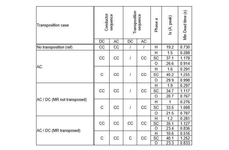
Table 5 - Line transposition simulations from Table 4 with additional fault cases, (H : Healthy ; SC : Short-circuited, O : Open)
In all transposition cases, when one phase is short-circuited, the SAC is much higher compared to the reference case, between 33.5 A to 40.2 A leading to a dead time always higher than 1 second. When the faulted phase is open, the SAC is still higher than the reference case value with an average magnitude of 24.2 A, resulting in a dead time of 856 ms. If all phases are not healthy, the benefit of line transposition is lost and the required dead time is unacceptably long. Line transposition is efficient to reduce the SAC and consequently dead time, but it is not reliable enough and has to be completed with another solution.
5.2.2. Line transposition and High-Speed Earthing Switches
Ss Since HVDC lines are interesting for long-distance transmission, it is highly possible that the existing AC line, candidate for the upgrade from AC to DC, would already be transposed. The HSES (High-Speed Earthing Switches) study was then directly conducted with transposed lines. Simulations were then conducted with the same additional fault states presented in section 5.2.1.2 with both transposition and HSES either on both line ends, or only one. The fault always remained at one of the worst locations: 50 km from the beginning.
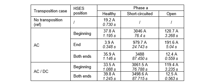
Table 6 - SAC (A, peak) and dead time (s) below for additional fault states with line transposition and HSES
Almost all values of the secondary arc presented in Table 6 lead to unacceptable dead times (more than 1 s). In case of a short-circuited phase, currents are too high and it may not be suitable to apply Equation 1. Moreover, switches need a time to open and close, which increases the dead time since HSES would have to close and open once the pole is opened by circuit breakers. The association of line transposition and HSES is to be avoided because it could even lead to permanent faults according to the values of SAC when the phase a is short-circuited.
5.2.3. Influence of the 4-legged shunt reactors of AC lines
The influence of the four-legged shunt reactors on the dead time and SAC is simulated. The reactors are installed on both ends of the AC system of the hybrid AC/DC line. By applying the method proposed in [21] at the configuration described in section 3, the calculated inductances values are (see Figure 5):
| Percentage of compensation | 85% | 70% |
|---|---|---|
Ls (H) | 2.6 | 3.1 |
Ln (H) | 1.7 | 4.3 |
5.2.3.1. Influence of the fault location
First, the influence of the fault location was studied along the line with 85% compensation four-legged shunt reactors and healthy phases. These simulations were conducted thrice for an un-transposed line, an AC-transposed line and for an AC/DC transposed line with MR included in the transposition. All conductors and transposition sequences were counter-clockwise. The fault location was changed every 25km.
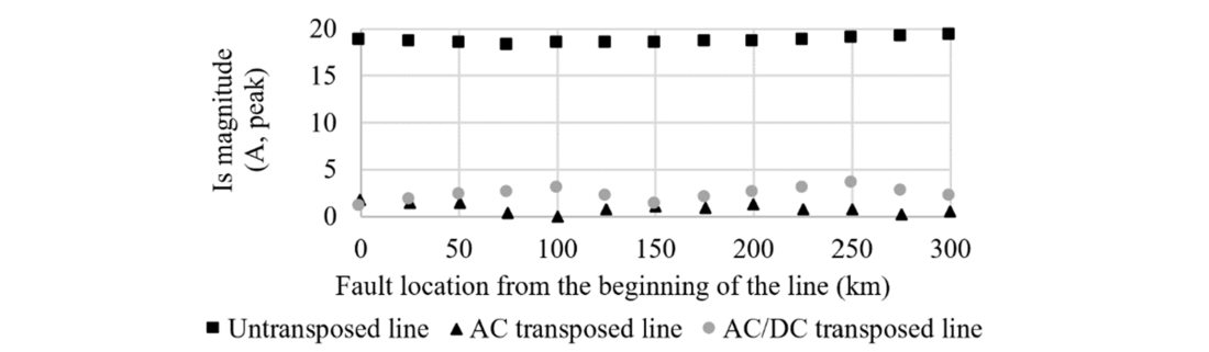
Figure 17 - Influence of fault location with four-legged shunt reactors
According to Figure 17, for the un-transposed and AC transposed line, the current variation is neglectable (less than 2 A) and it is considered not dependent on fault location at 18.7 A and 0.9 A (peak) respectively. For the AC/DC transposed line, the SAC is slightly dependent of the fault location (variation of 2.3 A peak) when the four-legged shunt reactors are installed on the line. In this case, the highest current happens at 250 km from the beginning of the line. This fault location was chosen for the rest of studies with reactors. Since it is highly probable that the upgraded line would already be transposed, only the un-transposed, for the sake of comparison, and hybrid AC/DC transposed line will be further studied.
5.2.3.2. Influence of phases’ health, line transposition and percentage of compensation
The following simulations study the influence of four-legged shunt reactors on lines with different configurations regarding line transposition, phases’ health and percentage of reactive power compensation.
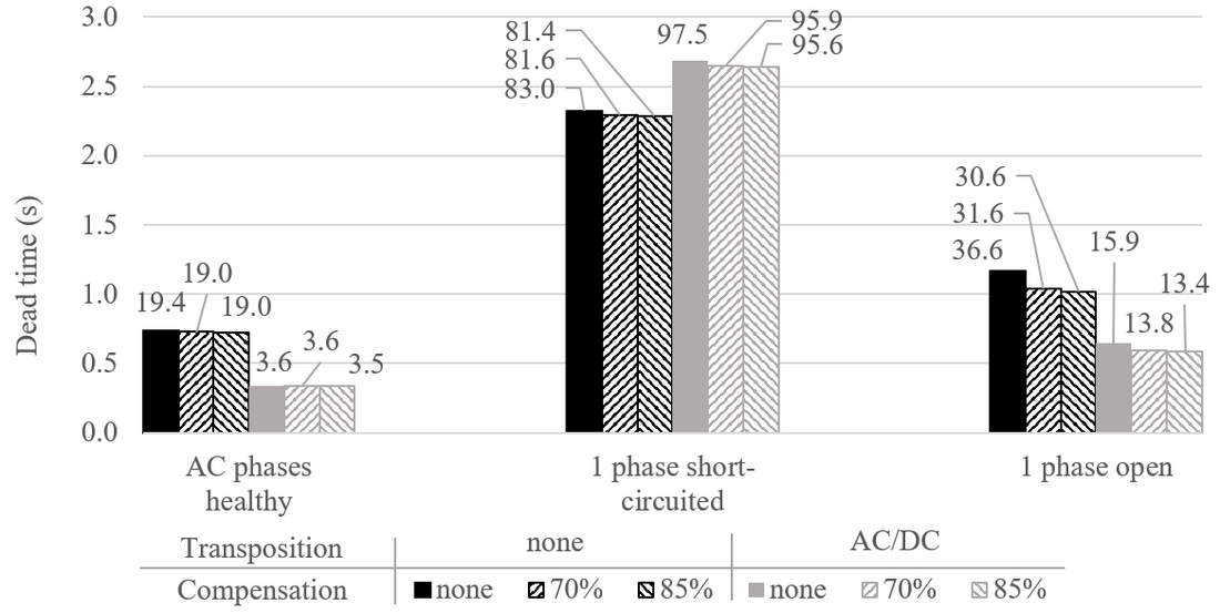
Figure 18 - Comparison of the required dead time to extinguish the secondary arc on a pole of a hybrid AC/DC line for different AC compensation, different phases health status and with or without line transposition. Labels are the corresponding SAC in A (peak)
According to Figure 18, the percentage of compensation makes no difference regarding the SAC. The presence of the four-legged shunt reactors only has a tiny influence when one phase is open. Then it reduces the SAC of 5.5A and 2.3A (dead times reduction of 140 ms and 50 ms) respectively when the line is un-transposed and transposed. The presence of the four-legged shunt reactors does not worsen the situation regarding the SAC and dead time.
5.2.3.3. Influence of the fourth reactor
From the 85% compensation case, the value of the fourth inductance (Ln) was varied from 0 to 10 H to see if it could be used to reduce the dead time. According to simulations, the fourth reactor value has no influence on the dead time except when one phase is opened without fourth reactor (increase of 3.4A). Consequently, from the DC point of view it is still better to use a fourth reactor.
The fourth reactor value cannot be adapted to reduce the dead time of a pole-to-ground fault on an AC/DC hybrid line.
6. Conclusions
The evaluation of the required dead time when a secondary arc occurs on a hybrid AC/DC line was performed through the SAC. A numerical expression of this current was calculated and validated via simulations for a line without metallic return. A sensitivity analysis was conducted to determine the influence of different line and system parameters on the SAC. The SAC increases mainly with the line length and the number of conductors per bundle. It is lower for some faulted pole location on the tower, with the presence of a sky wire, or with a higher arc resistance. Based on the assumptions of the study, transposition was found as the most efficient method to decrease SAC. The best transposition configurations to reduce the SAC of more than 90% (dead time order of value of 285 ms) are:
- AC line transposition, whatever phase and transposition sequence
- AC and DC line transposition, metallic return not transposed, whatever phase and transposition sequence
- AC and DC line transposition, metallic return transposed, whatever conductor sequence but same transposition sequence for AC and DC system.
The configuration AC and DC line transposition, metallic return transposed with opposite transposition sequence for AC and DC systems still reduces the SAC of 53%. Since it is less efficient it would be better to choose one of previously mentioned options. Line transposition with HSES should be avoided because this association of solutions worsen the SAC. The four-legged shunt reactors have no influence on the DC SAC. But, this means that it can be used on the AC side without any safety implications on DC SAC.
Line transposition is efficient as long as the phases are healthy. If there are not, another protection strategy should be defined. It could either be to open all AC and DC conductors or to make sure that the AC fault was cleared before considering reclosing the DC poles.
In future work AC and DC protection coordination could be studied to maximize the reduction of the dead time while ensuring continuity of service as much as possible on healthy conductors.
7. Appendix
7.1. Tower configuration
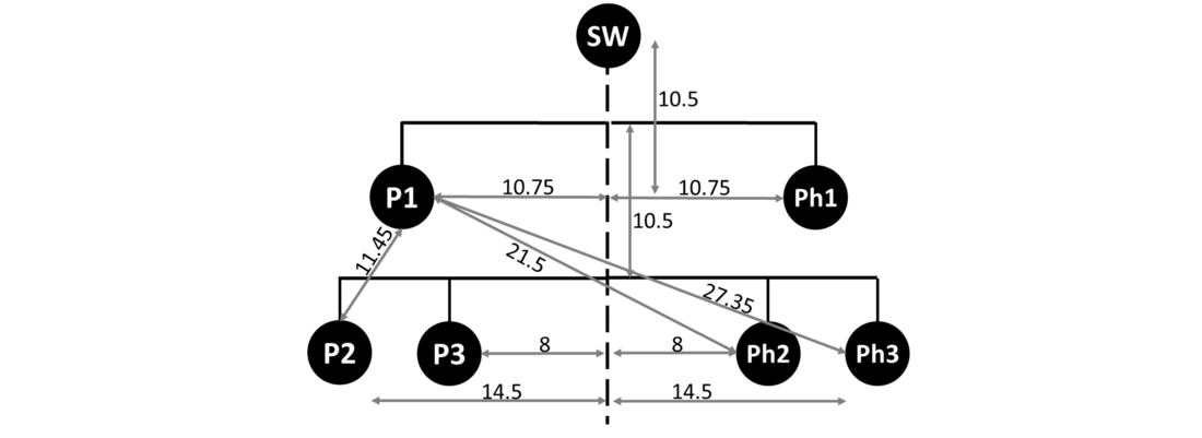
Figure 19 - Tower dimensions (distances are in m, SW : Sky Wire)
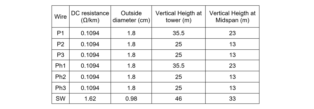
Table 8 - Conductors data
The zero and positive sequence susceptances of the AC system are respectively 0.4 mS and 1.5 mS.
7.2. Series impedances calculations
Series impedances represent everything that may limit the current in case of a short-circuit. They are calculated according to the IEC 60909 standard [25] that gives short-circuit expressions. Maximum acceptable short-circuit currents values are set in case of three AC phases isolated short-circuit () and in case of a single phase-to-ground short circuit (
).
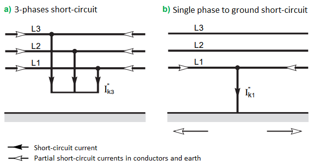
Figure 20 - Short-circuit currents' definition [25]
In the case of a short circuit far from electric machines, the expressions of initial short-circuit currents’ magnitude are:
(3)
(4)
With Un being the RMS voltage between phases, c is the voltage factor which is 1.1 to find the maximum current value, in the case of high voltage lines. Zo and Z1 are the zero and positive sequence impedances that define the series impedance. The maximum initial current values for both kinds of short-circuit are set to 13 kA. is then set to 19.5 Ω by Equation 3, both Equation 3 and Equation 4 lead to
. Assuming that Zo and Z1 are only inductive sets
to 19.5 Ω too.
7.3. Reference schemes settings
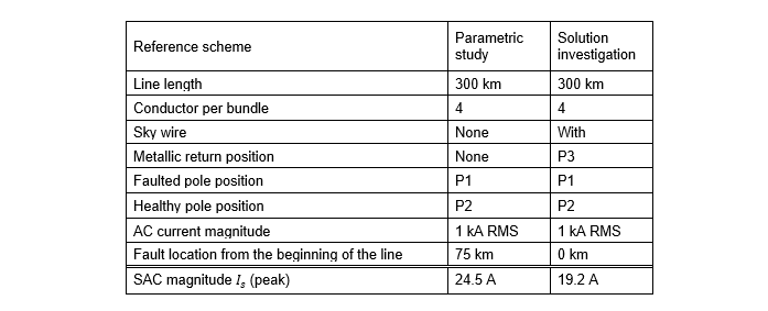
Table 9 - Reference schemes settings
7.4. Secondary arc expression
7.4.1. Without sky wire nor metallic return
The line is modelled directly in the faulted state : the circuit breakers are opened and the SAC flows to the earth. The following hypotheses are made :
- Line impedances, electromagnetic coupling, healthy pole, sky wire and metallic return are neglected
- AC conductors are almost identical to each other
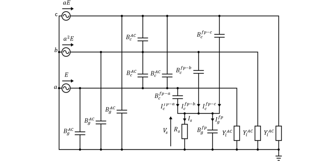
Figure 21 - Hybrid AC/DC line representation in faulted state
Leading to Equation 2:
The reference scheme built for the parametric study (Is = 24.5 A peak) validates the equation (Is = 24.04 A peak).
7.4.2. With sky wire
The fault happens at a tower location where the sky wire is earthed. The sky wire can then be considered as another conductor at 0V which can be "mixed" with the earth. On the scheme presented in Figure 21, the presence of the sky wire would add a susceptance in parallel with
between the faulted pole and the earth. Consequently, Equation 2, would be updated as follow:
7.5. Transposition parameters
- Transposition sequence: The physical rotation direction of phases between towers. It corresponds to the rotation direction that a conductor follows when the transposition happens on the tower : it could be either clockwise or counter-clockwise (see Figure 22).
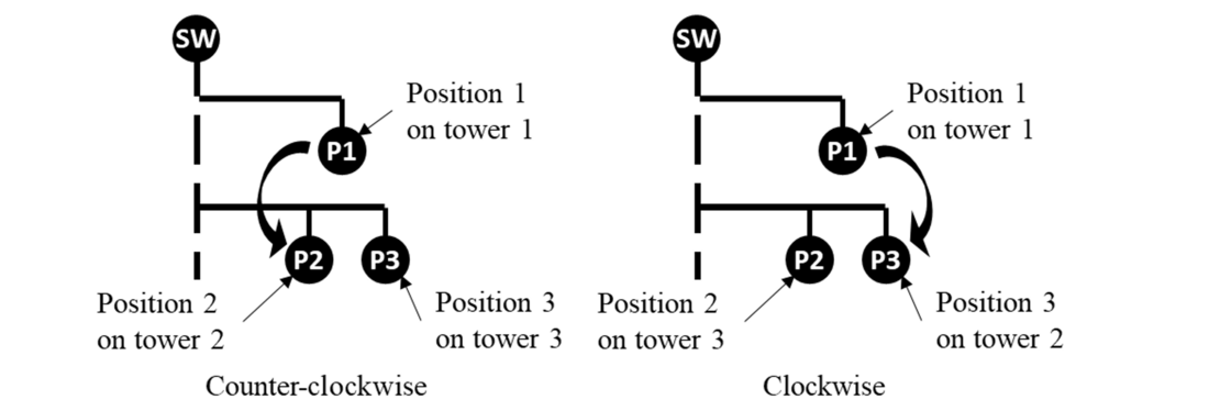
Figure 22 - Transposition sequence
- The conductor sequence : It is the positioning of phases (respectively the poles) regarding the others. This corresponds to which specific conductor each phase (pole) is connected to on an OHL. If the A, B, C (+, -, MR) order is considered, a phase (pole) sequence can be either clockwise or counter-clockwise (see Figure 22). This parameter is defined on lines independently of line transposition.
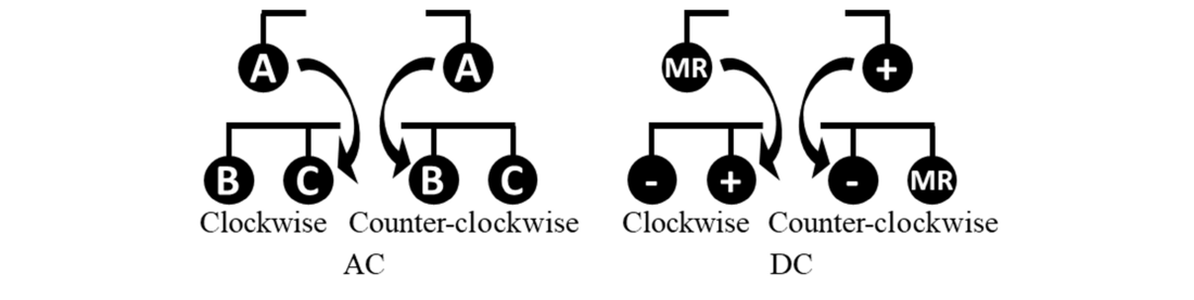
Figure 23 - Conductor sequence
Acknowledgment
This work was funded by SuperGrid Institute, an institute for the energetic transition (ITE). It is supported by the French government under the frame of “Investissements d’avenir”, No. ANE-ITE-002-01.
References
- V. L. Chartier, S. H. Sarkinen, R. D. Stearns, and A. L. Burns, ‘Investigation of corona and field effects of AC/DC hybrid transmission lines’, IEEE Trans. Power Appar. Syst., no. 1, pp. 72–80, 1981.
- M. Kizilcay, a Agdemir, and M. Losing, ‘Interaction of a HVDC System with 400kV AC systems on the same tower’, Proc. Int. Conf. Power Syst. Transients 2009 (IPST 2009), pp. 3–6, 2009.
- U. A. Khan, J.-G. Lee, S.-W. Lim, B.-W. Lee, Y.-G. Kim, and J. Sim, ‘A comparative study on electrical and thermal stress distribution across fundamental components of conventional and superconducting hybrid type HVDC circuit breakers’, in 2015 3rd International Conference on Electric Power Equipment–Switching Technology (ICEPE-ST), 2015, pp. 574–579.
- H. J. Haubrich, G. Hosemann, and R. Thomas, ‘Single-Phase Auto-Reclosing in Ehv Systems.’, in Int Conf on Large High-Voltage Electr Syst, 25th Sess, Bull, 1974, no. 1.
- emtp.com, ‘EMTP®Home’, 2021. https://www.emtp.com/ (accessed Dec. 10, 2021).
- ITU, ‘Protection against electromagnetic effects – Volume 3: Capactive, inductive and conductive coupling: physical theory and calculation methods’, 1990.
- Q. Sun, W. Shi, W. H. Siew, H. Liu, and Q. Li, ‘The induced overvoltage between UHV AC and DC transmission lines built on the same tower under fault conditions’, in 2009 44th International Universities Power Engineering Conference (UPEC), 2009, pp. 1–5.
- K. R. Ibrahim, O. Pischler, and U. Schichler, ‘Audible Noise and Corona Losses of DC Circuits on Hybrid Overhead Lines’, in 2019 54th International Universities Power Engineering Conference (UPEC), 2019, pp. 1–6.
- M. Gu, L. Meegahapola, and K. L. Wong, ‘Investigation of Factors Affecting the Critical Clearing Time of Hybrid AC/DC Power Systems’, in 2020 12th IEEE PES Asia-Pacific Power and Energy Engineering Conference (APPEEC), 2020, pp. 1–6.
- Y. Sekine, Y. Ichida, A. Nakamura, I. Kurihara, and H. Suzuki, ‘Asymmetrical four-legged reactor extinguishing secondary arc current for high-speed reclosing on UHV system’, in International Conference on Large High Voltage Electric Systems (CIGRE), 1984.
- C. D. Barker et al., ‘Multi-terminal operation of the South–West link HVDC scheme in Sweden’, in CIGRE Canada Conference, Montereal, Canada’, 2012.
- S.-H. Sohn et al., ‘Analysis of secondary arc extinction effects according to the application of shunt reactor and high speed grounding switches in transmission systems’, J. Int. Counc. Electr. Eng., vol. 4, no. 4, pp. 324–329, 2014.
- M. Kizilcay, G. Ban, L. Prikler, and P. Handl, ‘Interaction of the secondary arc with the transmission system during single-phase autoreclosure’, in 2003 IEEE Bologna Power Tech Conference Proceedings, 2003, vol. 2, pp. 7-pp.
- L. Prikler, G. Ban, M. Kizlicay, G. Tari, A. Tombor, and J. Zerenyi, ‘Influence of the Secondary Arc on the Operation of Single Phase Autoreclosure of the 400 kV interconnection between Hungary and Croatia’, J. Energy Energ., vol. 59, no. 1–4, p. 0, 2010.
- J. B. Mooney, ‘Economic analysis and justification for transmission line transposition’, in IEEE PES T&D 2010, 2010, pp. 1–5.
- B. Li, Y. Li, J. He, and Y. Zheng, ‘Multi-circuit transmission lines’, in Protection Technologies of Ultra-High-Voltage AC Transmission Systems, Academic Press, 2020.
- C. Romeis, J. Schindler, J. Jaeger, M. Luther, K. Steckler, and T. Keil, ‘Induced voltages on HVDC systems by HVAC systems at the same support structure due to capacitive and inductive coupling’, in 11th IET International Conference on AC and DC Power Transmission, 2015, pp. 1–7, doi: 10.1049/cp.2015.0019.
- Z. Xu, Y. Xiaoqing, and X. Zhenyu, ‘HSGS Investigation for Limiting the Secondary Arc on UHV Parallel Lines’, in The 2nd International Conference on Computer Application and System Modeling, 2012.
- C. H. Kim and S. P. Ahn, ‘The simulation of high speed grounding switches for the rapid secondary arc extinction on 765 kV transmission lines’, in Proc. of the Int’l Conf. on Power Systems Transients, Hungary, 1999, pp. 173–178.
- CIGRE Study Commitee A3, Technical Requirements for Substation Equipment Exceeding 800 KV: Field Experience and Technical Specifications of Substation Equipment Up to 1200 KV. CIGRÉ, 2008.
- E. Nashawati, N. Fischer, B. Le, and D. Taylor, ‘Impacts of Shunt Reactors on Transmission Line Protection’, 38th Annu. West. Prot. Relay Conf., no. November, pp. 1–16, 2011.
- E. W. Kimbark, ‘Suppression of ground-fault arcs on single-pole-switched EHV lines by shunt reactors’, IEEE Trans. Power Appar. Syst., vol. 83, no. 3, pp. 285–290, 1964.
- H. A. Peterson and N. V Dravid, ‘A method for reducing dead time for single-phase reclosing in EHV transmission’, IEEE Trans. Power Appar. Syst., no. 4, pp. 286–292, 1969.
- C. Neumann, B. Rusek, S. Steevens, and K.-H. Weck, ‘Design and layout of AC-DC hybrid lines’, Cigre Auckl. Symp., pp. 1–9, 2013.
- B. de Metz-Noblat, F. Dumas, and C. Poulain, ‘Cahier technique n 158: Calcul des courants de court-circuit’, Schneider Electr. CT, vol. 158, 2005.
- J. Schindler, C. Romeis, and J. Jaeger, ‘Secondary arc current during DC auto reclosing in multisectional AC/DC hybrid lines’, IEEE Trans. Power Deliv., vol. 33, no. 1, pp. 489–496, 2017.
- B. Sander, J. Lundquist, I. Gutman, C. Neumann, B. Rusek, and K. H. Weck, ‘Conversion of AC multi-circuit lines to AC-DC hybrid lines with respect to the environmental impact’, Cigre Sess. Paris, vol. 2, no. 105, 2014.