Theoretical Design of Economic Incentive in Demand Response Programs
Authors
H. TAKANO, N. YOSHIDA - Gifu University, Japan
H. ASANO - Gifu University, Japan & Central Research Institute of Electric Power Industry, Japan

Summary
Demand response (DR) program is a framework that changes electricity consuming patterns by changes of electricity rate or incentive payments. There are two major types in the DR programs: one is the price-based program, and the other is the incentive-based one. Time of use, real time pricing and critical peak pricing are typical examples of the former type. Electricity rates in these programs become expensive during the periods of high electricity costs or the periods when the power grid is in critical conditions (peak periods), in comparison with the other periods (off-peak periods). On the other hand, peak time rebate and critical peak rebate are included in the latter type. In the incentive-based programs, power suppliers (or power producers, retailers, etc.) reward consumers, who respond to requests of the DR, with money rebates. Since either type of the DR programs brings controllability in demand side without huge investment costs, they are highly expected as an efficient alternative to the traditional power supply-demand balancing operations. In fact, many DR-related studies have been actively progressing, as well as demonstrative field tests. However, there are still significant issues in the actual DR programs on setting of the electricity rates and the rebate levels while ensuring their resources. These values have been decided relying on knowledge and experience of operators and experimental results, and it makes difficulties on the verification for appropriateness of the setting.
The authors propose a theoretical approach that calculates the optimal values of the electricity rate and the rebate level in DR programs based on the framework of social welfare maximization (SWM). The SWM framework has often been applied to represent models of electricity markets but is used for evaluating contributions of the DR in this study. In the authors’ proposal, first, the surplus functions of the power suppliers and the consumers are represented, and the power supply-demand balancing operation is formulated in the style of an SWM problem. This process makes the contributions of the DR measurable as increment/decrement of the surplus functions. Next, acceptable ranges of the electricity rates and the rebate levels are derived, and finally, the optimal values of the electricity rate and the rebate level are defined from the standpoint of minimal burden on the DR programs. Through numerical simulations and discussion on their results, the validity of the authors’ proposal was verified. The numerical simulation models were constructed by using a widely used fuel cost function and actually measured data of the electricity consumption. Although the assumed models have room for discussion on its appropriateness, the results of numerical simulations captured trends in leading studies for the DR programs.
Keywords
Demand Response Program - Electricity Rate - Rebate Level - Social Welfare Maximization - Surplus Function - Lagrange Relaxation - Karush-Kuhn-Tucker Condition1. Introduction
Demand response (DR) is to intentionally change electricity consuming patterns by changes in electricity rate or incentive payments [1]. The DR programs are classified into the following two types: one is the price-based program, and the other is the incentive-based one. The typical examples of the former type are time of use (TOU), real time pricing (RTP) and critical peak pricing (CPP). In the price-based programs, electricity rates become expensive during the periods of high electricity costs or the periods when the power grid is in critical conditions (peak periods), in comparison with the other periods (off-peak periods). The latter type, on the other hand, includes peak time rebate (PTR) and critical peak rebate (CPR). In the incentive-based programs, power suppliers (or power producers, retailers, etc.) reward consumers, who respond to requests in the DR programs, with money rebate. Any of the DR programs give controllability in the demand side without huge investment costs in power plants or facilities, and thus, they have been attracting attention as one of the most economical and sustainable alternatives to the traditional power supply-demand balancing operations. Moreover, many DR-related studies and developments have been actively carried out [2-4], as well as demonstrative field tests.
There are various studies contributing to design of the DR programs. In [5], states of DR-related activities are analyzed with highlighting deregulation in electric power markets. The authors also set evaluation indices for the DR programs and discuss their effects focusing on the electricity prices. The authors of [6] review the means that power suppliers induce their preferable electricity consumption in DR programs. Several mathematical problem frameworks and models are summarized, and their solution techniques are discussed in this literature. In [7], DR programs are organized from the viewpoints of their decision variables, control mechanisms, and motivations offered to changes in the electricity consuming pattern. In addition, several models for optimizing control strategies in the DR programs are categorized in association with the application targets. The authors of [8] focus on price-based DR programs and evaluate their advantages and disadvantages with experimental results. This literature includes a review of case study results in several countries. Similarly, the authors of [9] summarized results of case studies and analyzed them to discuss preferable electricity rates setting in the price-based programs.
Although these literatures provide useful information, the actual DR programs still have significant issues on their theoretical design. In fact, the electricity rates and the rebate levels are decided relying on knowledge and experience of operators and experimental results [10-14], and as a result, it becomes difficult to discuss appropriateness on setting of the electricity rates and the rebate levels. For these reasons, development of design techniques for efficient DR programs is now regarded as a crucial component on advancing technologies for the power grid management.
This paper presents a theoretical approach that calculates the electricity rates and the rebate levels in DR programs. The authors’ proposal builds upon the framework of social welfare maximization (SWM), which has often been used to represent models of electricity markets [6,7,15-18]. First, the authors set the surplus functions of the power suppliers and the consumers, and then, formulate the power supply-demand balancing operations as an SWM problem. By the process, contributions of the DR to the operations become measurable as increment/decrement in the surplus functions. Next, acceptable ranges of the electricity rate and the rebate level are derived from the DR-originated changes in the surplus functions. Furthermore, the ideal, optimal values of the electricity rate and the rebate level are defined in consideration of burden accompanying with the DR programs. The basis of the above proposal was previously discussed in [19,20]. However, these works hold the assumption that the power suppliers know the standard values of electricity consumption without the DR, and it is not the case in operations of the actual power grids. In this paper, the standard is replaced with readily available information, and finally, the practical, optimal values of the electricity rate and the rebate level are calculated.
The validity of the authors’ proposal is verified through numerical simulations on models constructed by using a widely used fuel cost function and actually measured data of the electricity consumption.
2. Representation of power supply-demand balancing operation
SWM framework is formulated as the problem that maximizes the weighted sum of surplus functions in a society without regarding to how the profit distributed in each member of the society [21-23]. The authors classify the members of society into the power suppliers (or power producers, retailers, etc.) and the consumers, and then, define the social welfare function as:
(1)
where ? is the time slot (?=1,⋯,?); ? is the number assigned to the power suppliers (?=1,⋯,?); ? is the number assigned to the consumers (?=1,⋯,?); ?1(∙) is the surplus function of the power suppliers; ?2(∙) is the surplus function of the consumers; ??,? is the electric power fed from the power supplier ?, and an element of vector ??; ??,? is the power consumption in the consumer ?, and an element of vector ??; ? is the weighting coefficient.
The suppliers’ surplus is treated as the sum of the revenue from selling electricity (suppliers’ utility) and the operational costs in the power supply, while the consumers’ one as the sum of the satisfaction acquired in exchange for consuming electricity (consumers’ utility) and the electricity costs [6,24]. Besides, in design of the DR mechanisms, it can be regarded each of the power suppliers and the consumers as aggregated ones. Hence their surplus functions are expressed with:
(2)
(3)
where ?1(∙) is the operational cost function of the power suppliers; ?2(∙) is the price-converted utility function of the consumers; ?? is the electricity rate.
In Equations (2) and (3), all units of each term are unified to the price, and in this case, the coefficient ? equals to 1. The SWM problem can be formulated as:
(4)
(5)
(6)
(7)
where ?max and ?min are the maximum and the minimum values of the power supply.
Equation (6) shows the balance of power supply and demand, and Equation (7) restricts controllability of the power supply depending on specifications of the target power grid, e.g., the maximum and the minimum outputs of power generation units. That is, the optimal solution of the formulated SWM problem represents the power supply-demand operations that maximize the social welfare. In the case that Equation (5) is a convex function, we can apply Lagrange relaxation [6,25,26], and Lagrange multipliers correspond to shadow prices. Lagrange function and Karush-Kuhn-Tucker (KKT) conditions are represented as:
(8)
(9)
where ??, ?1,? and ?2,? are the Lagrange multipliers.
3. Calculation of electricity rates and rebate levels
In the DR programs, the power suppliers change the electricity rate or the rebate level for bringing the electricity consumption closer to the preferable on the power supply-demand management. The target electricity consumption in a DR program is defined as:
(10)
where ?? is the actual electricity consumption without the DR, which is the standard for the electricity consumption; Δ?? is the change in the electricity consumption after the DR.
Under the following assumption, we can calculate acceptable ranges of the electricity rates and the rebate levels, and the optimal values of them:
(Assumption 1) Consumers buy electricity to maximize their surplus function. This assumption activates Equation (11) derived by Equations (8) and (9).
(11)
where ?? is the actual electricity rate without the DR, which is the standard for the unit price of electric power.
To simplify the formulation, discussion on the time-dependent dynamics in the operations of power grids are excluded from this paper.
3.1. Definition of Ideal Electricity Rate and Its Calculation
The power suppliers decide the electricity rates in the price-based DR programs to control the electricity consumption. The ideal, optimal electricity rate leading to the preferable electricity consumption is temporary set as:
(12)
where Δ?? is the change in the electricity rate for the DR request.
According to Equations (2) and (3), the DR-originated changes are calculated as:
(13)
(14)
where Δ?1,? is the change in the operational cost by the is the change in the consumers’ utility by the
.
If the power suppliers set a higher electricity rate than the standard ??, hereafter , the consumers’ surplus decreases depending on Equation (14), and the electricity consumption is reduced (Δ??>0). On the other hand, the electricity consumption is promoted (Δ??<0) by setting the electricity rate lower than the standard, hereafter
.
Each surplus of the power suppliers and the consumers must be larger than zero regardless of the . Since the power suppliers request the DR to improve their economic efficiency, the change in the surplus of the power suppliers becomes larger than zero (Δ?1,?>0). Meanwhile, without any incentive, the change in the surplus of the consumers is in negative (Δ?2,?<0). Under these boundary conditions and Assumption 1, the acceptable ranges of
and
are respectively derived as:
(15)
By setting the electricity rate in the ranges of Equation (15), the DR gives the positive economic impact to the power suppliers. Meanwhile, the price-based DR programs induce only burden to the consumers. Based on them, the authors define the ideal electricity rate as:
(16)
3.2. Definition of Ideal Rebate Level and Its Calculation
The surplus of the consumers decreases in response to their contributions to the DR programs. This is because the consumers must accept lower utility than that acquired at the standard electricity consumption. In the incentive-based DR programs, the DR-originated changes in the surplus functions of the power suppliers and the consumers are calculated as:
(17)
(18)
These equations are similar to Equations (13) and (14); however, the electricity rates are fixed at ?? in the incentive-based programs. Although the consumers accept lower utility, their surplus recovers to its original level by compensating the decrement of Equation (18). Hence the acceptable range of the unit price of money rebate ?? is set as:
(19)
This condition indicates in which the DR request has no negative impact on both the power suppliers and consumers. In this paper, the ideal, optimal rebate level is set to induce the most active cooperation in the DR programs as:
(20)
3.3. Practical Values of Electricity Rate and Rebate Level
If the power suppliers know the true standard ??, the DR programs can be optimally designed by calculating Equations (16) and (20). However, it is not the case since the true standard is not measurable in the actual power grid operations. The only available is its estimated one represented as:
(21)
where ??? is the deviation from the true standard ??.
In Japan, the committee of Energy Resource Aggregation Business (ERAB committee), which was established by the Ministry of Economy, Trade and Industry in 2016, defines ‘standard baseline’ based on the representative day methods (High X of Y methods) [27] in the guidelines of ERAB [28]. The ERAB baselines, unlike the true standard, are the estimated values, but can be calculated using the historical record of electricity consumption as:
(22)
where ? is the ranking (?=1,2,…,?,…,?); ??,? is the ?-th value of electricity consumption data sorted in descending order for ? days.
As shown in Equation (16), the optimal electricity rates do not directly depend on the true standard, and therefore, so this definition can practically be used in the price-based DR programs. In contrast, the incentive-based programs require the true standard in calculation of the optimal rebate level, so the deviation ??? makes a difference in Equation (20). The practical, optimal rebate level is calculated by replacing ?? with as:
(23)
where is the change in the electricity consumption after the
is the change in the operational cost by the
.
The deviation not only causes a gap between Equations (20) and (23) but can also indirectly change the calculation of the electricity rates. Detailed discussions on these issues remain as a future work of this study.
4. Numerical simulations and discussion on their results
The validity of the authors’ proposal was verified through numerical simulations and discussion on their results. The functions of operational cost and consumers’ utility were made by using a widely used fuel cost function and an actual record of the electricity consumption. The standard electricity rates were assumed to 23.90 JPY/kWh (??=23.90, for ∀?) which is the Japanese annual average in 2015.
4.1. Numerical Simulation Model
Thermal power generation units take a large portion in the power supply, e.g., approximately 91 % on 2017 in Japan [29], and their fuel costs have often been approximated as quadratic functions by means of their generating power [30-32]. The authors set the fuel cost and the operational cost functions by Equation (24) under the following assumptions [20]:
(Assumption 2) Total operational cost in the power supply is approximated as the quadratic function relying on the fuel costs of thermal power units.
(Assumption 3) The power suppliers decide the electricity rate to maximize their surplus function at the annual average of electricity consumption (103.94 kW in this paper).
(24)
where ? and ? are the coefficients of the operational cost function.
In the numerical simulations, the authors set the coefficients ? and ? to 1.15×10⁻¹ and 2.29×10⁻⁴, respectively.
In contrast, consumers’ utility has been approximated by several functions, such as logarithmic or sigmoidal functions [19,20,33-35]. With reference to [20], approximated functions of hourly cumulative frequency distributions of the electricity consumption were regarded as the functions of hourly utility in this paper. Figure 1 shows the profiles of daily total electricity consumption of 500 households measured by smart power meters and the calculated ERAB baselines. These are samples including period of the highest or the lowest electricity consumption for one year.
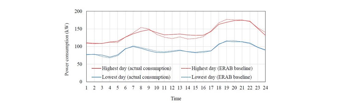
Figure 1 - Profiles of total electricity consumption of 500 households
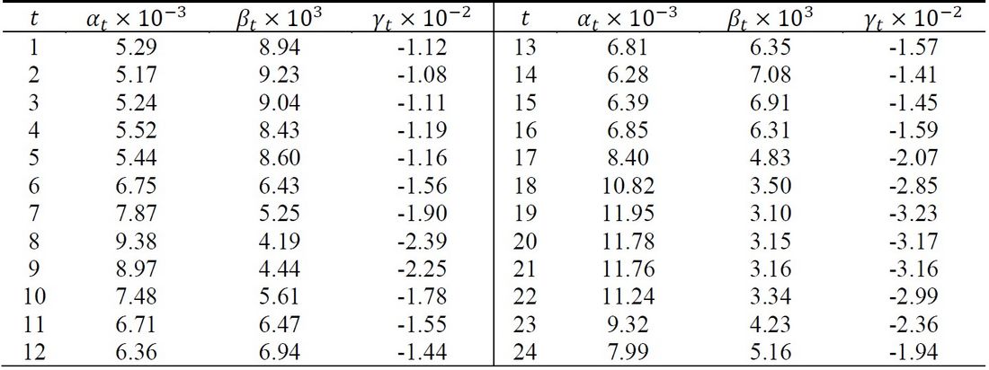
Table 1 - Coefficients of consumers’ utility on highest day of electricity consumption
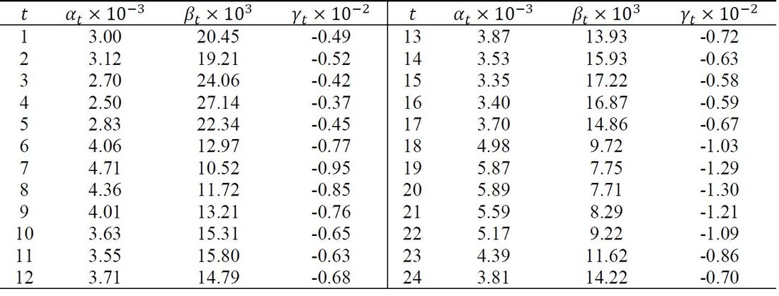
Table 2 - Coefficients of consumers’ utility on lowest day of electricity consumption
The unit of approximated functions was converted into the price based on Assumption 4, and as a result, Equation (25) was given as the functions of consumers’ utility and surplus.
(Assumption 4) Maximum values of each daily consumers’ surplus is equal to the maximum value in the surplus function of the power suppliers.
(25)
where ??, ?? and ?? is the coefficients of the price-converted consumers’ utility.
Tables 1 and 2 summarize the coefficients ??, ?? and ?? based on the ERAB baselines. For further details of the calculation process of the functions, refer to [20].
4.2. Numerical Simulation Results
The practical, optimal electricity rates, , and rebate levels,
, were calculated under the following scenarios:
(Scenario 1) The power suppliers request to reduce the electricity consumption at any time slot in the day of the highest electricity consumption.
(Scenario 2) The power suppliers encourage the electricity consumption at any time slot in the day of the lowest electricity consumption.
As the basis of comparison, the ideal, optimal electricity rates, , and rebate levels,
, were calculated by using the functions of utility and surplus of the consumers based on the true profiles. Equation (16) is applicable to the practical, optimal electricity rates; however, the ERAB-based functions of utility and surplus of the consumers are not the same as the true profile-based ones. This is the reason why the authors additionally set
.
4.2.1. Results for Price-based Demand Response
Tables 3 and 4 summarize the calculation results of the case that the power suppliers set the DR target as 1 % increase (Scenario 1) or decrease (Scenario 2) as compared to the (assumed) standard of electricity consumption.

Table 3 - Numerical simulation results on highest day of electricity consumption
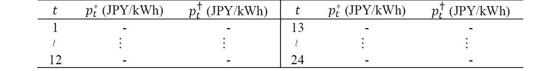
Table 4 - Numerical simulation results on lowest day of electricity consumption (JPY/kWh)
In Scenario 1, after calculating their acceptable ranges, the ideal and practical, optimal electricity rates were obtained. As shown in Table 3, both optimal electricity rates became slightly larger than the standard electricity rate (23.90 JPY/kWh), and the differences between and
were sufficiently small. On the other hand, in Scenario 2, both optimal electricity rates became smaller than the lower bound of the acceptable ranges. It means that, as shown in Table 4, the power suppliers could not request the DR because the increment of the power suppliers’ surplus was too small as compared to its decrement by the reduction in the electricity rates.
In the numerical simulations, the authors made the operational cost function of the power suppliers relying on the fuel costs of thermal power units. However, in the actual operations, the other factors such as surplus power of renewable energy sources have influences on the operational cost. If we reflect them appropriately in the numerical simulation model, the results of Scenario 2 can be activated.
4.2.2. Results for Incentive-based Demand Response
Tables 5 and 6 summarize the calculation results of the case that the power suppliers set the DR target as 1 % increase (Scenario 1) or decrease (Scenario 2) as compared to the (assumed) standard of electricity consumption.
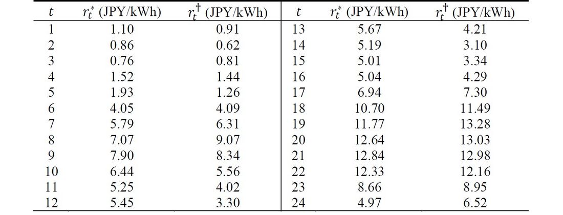
Table 5 - Numerical simulation results on highest day of electricity consumption (JPY/kWh)
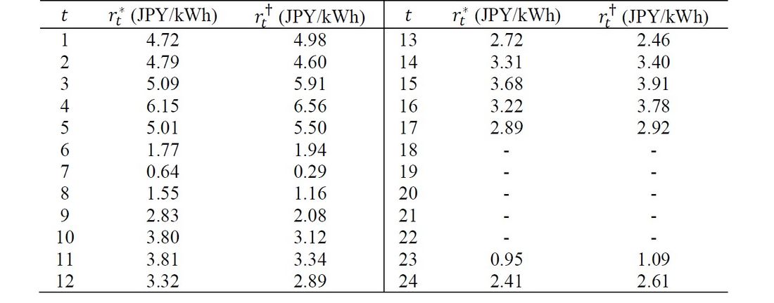
Table 6 - Numerical simulation results on lowest day of electricity consumption (JPY/kWh)
In Scenario 1, the practical rebate levels were in the range of 0.62 (?=2) to 13.28 (?=19) JPY/kWh, while the ideal rebate levels were in the range of 0.76 (?=3) to 12.84 (?=21) JPY/kWh. As shown in Fig. 1, the time slots 19 and 21 were the peak periods in true profile and ERAB baselines, respectively. In Scenario 2, the practical rebate levels were in the range of 0.29 (?=7) to 6.56 (?=4) JPY/kWh, while the ideal rebate levels were in the range of 0.64 (?=7) to 6.15 (?=4) JPY/kWh. The time slot 4 was the nadir period in both of true profile and ERAB baselines. During the period of 18:00 to 22:00, the optimal rebate levels became smaller than the lower bound of the acceptable ranges. This is because the electricity consumption (both of true values and ERAB baselines) exceeded the annual average of electricity consumption (103.87 kW), and as a result, the increase of the electricity consumption led to the negative economic impact to the power suppliers. As shown in Table 5, there were differences between and
unlike the calculation results of the electricity rates. It indicates that the rebate levels are more sensitive to changes in electricity consumption than the electricity rates. As mentioned earlier, the differences ??? brought gaps in the actual responses of the consumers, so it becomes important the discussion on how we should compensate the differences.
5. Conclusions
The authors proposed a theoretical approach calculating the electricity rates and the rebate levels in DR programs based on the SWM framework. In the authors’ proposal, first, the surplus functions of the power suppliers and the consumers were set, and then, the power supply-demand balancing operation was represented under the SWM framework. Next, the authors derived the acceptable conditions for price-based DR programs as (15) and for incentive-based programs as (19). Besides, the ideal, optimal values of electricity prices and rebate levels were defined as (16) and (20), respectively, in consideration of the DR-originated burden on the society. These were originally designed under the assumption that the power suppliers know the true standard of the DR programs; however, it does not apply to operations of the actual power grids. Therefore, in Subsection 3.3, the authors replaced the true standard with readily available information.
Through the numerical simulations, the validity of the authors’ proposal was verified. As shown in Section 4, the calculated electricity rates and rebate levels became smaller than those applied in the demonstrative field tests. This is because the calculation results were strongly dependent on the surplus functions of the power suppliers and the consumers, as described in Section 3. In other words, the assumed surplus functions have room for discussion on their appropriateness. However, the results of the numerical simulations reflected controllability in the electricity consumption, and we can conclude that the authors’ proposal functioned appropriately.
In future works, appropriateness of the assumed surplus functions will be discussed in more details. Furthermore, measures for compensating the gaps originated from the deviation ??? in Equation (21) will be considered.
Acknowledgements
This research was partly funded by the Japan Society for the Promotion of Science (JSPS; grant number: 19K04325).
References
- Palensky, P.; Dietrich, D. Demand side Management: Demand Response, Intelligent Energy Systems, and Smart Loads. IEEE Trans. Industr. Inform. 2015, 7(3), 381-388.
- Asano, H.; Nagata, Y. A Survey of Demand Response and Research Activities at CRIEPI. Review of Electricity Economics 2015, 62, 1-7. (In Japanese.)
- Siano, P. Demand Response and Smart Grids - A Survey. Renew. Sust. Energy Rev. 2014, 30, 461-478.
- Meyabadi, A.F.; Deihimi, M.H. A Review of Demand-side Management: Reconsidering Theoretical Framework. Renew. Sust. Energy Rev. 2017, 80, 367-379.
- Albadi, M.H.; El-Saadany, E.F. A Summary of Demand Response in Electricity Markets. Electr. Power Syst. Res. 2008, 78, 1989-1996.
- Deng, R.; Yang, Z.; Chow, M. Y.; Chen, J. A Survey on Demand Response in Smart Grids: Mathematical Models and Approaches. IEEE Trans. Industr. Inform. 2015, 11(3), 570-582.
- Vardakas, J.S.; Zorba, N.; Verikoukis, C.V. A Survey on Demand Response Programs in Smart Grids: Pricing Methods and Optimization Algorithms. IEEE Trans. Commun. Surv. Tutor. 2015, 17(1), 152-178.
- Yan, X.; Ozturk, Y; Hu, Z.; Song, Y. A Review on Price-Driven Residential Demand Response. Renew. Sust. Energy Rev. 2018, 96, 411-419.
- Faruqui, A. and Bourbonnais, C. The Tariffs of Tomorrow. IEEE Power & Energy Magazine 2020, 18-25.
- Faruqui, A.; Segucu, S. Household Response to Dynamic Pricing of Electricity: A Survey of 15 Experiments. J. Regul. Econ. 2010, 38, 193-225.
- Heter, K.; Wayland, S. Residential Response to Critical-Peak Pricing of Electricity: California Evidence. Energy 2010, 35(4), 1561-1567.
- Erucsibm, T. Households’ Self-Selection of Dynamic Electricity Tariffs. Appl. Energy 2011, 88, 2541-2547.
- Bartusch, C.; Wallin, F.; Odlare, M; Vassileva, I.; Wester, L. Introducing a Demand-based Electricity Distribution Tariff in the Residential Sector: Demand Response and Customer Perception. Energy Policy 2011, 39, 5008-5025.
- Kawamura, K.; Doki, T.; Oono, Y.; Takano, H.; Murata, J. Analysis of Field Test Results and Proposal of Sustainable Demand Peak Reduction in Demand Response Programs for Residential Consumers. IEEJ Trans. Electron. Inf. Syst. 2017, 137(1), 96-105. (In Japanese.)
- Zou, X. Double-sided Auction Mechanism Design in Electricity based on Maximizing Social Welfare. Energy Policy 2009, 37(11), 4231-4329.
- Yang, P.; Tang, G.; Nehorai, A. A Game-Theoretic Approach for Optimal Time-of-Use Electricity Pricing. IEEE Trans. Power Syst. 2013, 28(2), 884-892.
- Li, N.; Chen, L.; Dahleh, M.A. Demand Response Using Linear Supply Function Bidding. IEEE Trans. Smart Grid 2015, 6(4), 1827-1838.
- Sorin, E.; Bobo L.; Pinson, P, Consensus-Based Approach to Peer-to-Peer Electricity Markets with Product Differentiation. IEEE Trans. Power Syst. 2019, 34(2), 994-1004.
- Takano, H.; Tanonaka, N.; Kikuda, S.; Ohara, A. A Design Method for Incentive-based Demand Response Programs Based on a Framework of Social Welfare Maximization. IFAC-PapersOnLine 2018, 51(28),374-379.
- Takano, H.; Yoshida, N.; Asano, H.; Hagishima, A; Tuyen, N.D. Calculation Method for Electricity Price and Rebate Level in Demand Response Programs. Appl. Sci. 2021, 11(15), 6871.
- Luenberger, D.G. Microeconomics Theory. McGraw-Hill: NY, USA, 1995.
- Perloff, J.M. Microeconomics, Second Edition. Addison-Wesley: MA, USA, 2001.
- Hausman, D.; McPherson, M.; Sats, D. Economic Analysis, Moral Philosophy, and Public Policy, Third Edition. Cambridge University Press: Cambridge, UK, 2016.
- Liu, H.; Shen, Y.; Zabinsky, Z.B.; Liu, C.C.; Courts, A.; Joo, S.K. Social Welfare Maximization in Transmission Enhancement Considering Network Congestion. IEEE Trans. Power Syst. 2008, 23(3), 1105-1114.
- Baharlouei, Z.; Hashemi, M.; Narimani, H.; Mohsenian-Rad, H. Achieving Optimality and Fairness in Autonomous Demand Response: Benchmarks and Billing Mechanisms. IEEE Trans. Smart Grid 2013, 4(2), 968-975.
- Wang, H.; Gao, Y. Real-Time Pricing Method for Smart Grids based on Complementarity Problem. J. Mod. Power Syst. Clean Energy 2019, 7(5), 1280-1293.
- EnerNOC. The Demand Response Baseline. White Paper. https://library.cee1.org/sites/default/files/library/10774/CEE_EvalDRBaseline_2011.pdf (Accessed on 1 December 2021)
- Ministry of Economy, Trade and Industry. Guidelines for Energy Resource Aggregation Business. https://www.meti.go.jp/press/2020/06/20200601001/20200601001-1.pdf (Accessed on 1 December 2021) (In Japanese.)
- Agency for Natural Resources and Energy. Japan’s Energy White Paper 2020. https://www.enecho.meti.go.jp/about/whitepaper/ (Accessed on 1 December 2021) (In Japanese.)
- Hobbs, B.F.; Rothkopf, M.H.; O’Neill, R.P.; Chao, H.P. The Next Generation of Electric Power Unit Commitment Models.; Springer: Dordrecht, Netherlands, 2001.
- Padhy, N.P. Unit Commitment - A Bibliographical Survey. IEEE Trans. Power Syst. 2004, 19(2), 1196-1205.
- Zheng, Q.P.; Wang, J.; Liu, A.L. Stochastic Optimization for Unit Commitment - A Review. IEEE Trans. Power Syst. 2015, 30(4), 1913-1924
- Wang, L.; Wang, Z.; Yang, R. Intelligent Multiagent Control System for Energy and Comfort Management in Smart and Sustainable Buildings. IEEE Trans. Smart Grid 2012, 3(2), 605-617.
- Li, D.; Chiu, W.; Sun, H.; Poor, H.V. Multiobjective Optimization for Demand Side Management Program in Smart Grid. IEEE Trans. Industr. Inform. 2018, 14(4), 1482-1490.
- Patnam, B.S.K.; Pindoriya, N.M. Demand Response in Consumer-Centric Electricity Market: Mathematical Models and Optimization Problems. Electr. Power Syst. Res. 2021, Vol. 193, pp. 1-18.