Synthetic Data – A Solution to Train Diagnostic Systems for High-Voltage Equipment without Fault-Condition Measurements
Authors
J.N. KAHLEN - RWTH Aachen University
A.MUHLBEIER - BatterieIngenieure GmbH
M. ANDRES, A. MOSER - RWTH Aachen University
B. RUSEK, D. UNGER, K. KLEINEKORTE - Amprion GmbH

Summary
Downtimes of high-voltage equipment can be reduced by detecting abnormalities before faults occur, a task that can be performed by machine-learning (ML) diagnostic systems. Training such diagnostic systems requires data containing fault conditions. However, fault-condition measurements are often not available due to low fault rates. This raises the question of whether ML-diagnostic systems trained with synthetic data are valid predictors for real applications.
In this paper, synthetic data is generated with digital simulations of normal- and fault conditions of a high-voltage pantograph disconnector to train multiple ML-diagnostic systems. A system selection is executed using normal-condition measurements and the synthetic data only. Finally, the performance of the selected systems is evaluated with measurements of a disconnector with additional weight load.
The results show that most of the ML-systems trained with synthetic data are capable to detect the fault conditions. The systems based on artificial neural networks show the best diagnostic performance.
Keywords
Fault detection - fault diagnosis - fault simulation - machine learning - power engineering1. Introduction
To provide a safe, reliable and powerful electrical grid, a network operator has to take on a range of duties and responsibilities. In Germany, such obligations are defined by the National Electricity Act (EnWG). According to §12 and §13 of the EnWG, the network operator is obliged to provide a safe and reliable grid – both in the national framework and where international tie lines are concerned [1].
The downtimes of high-voltage equipment can be reduced by using monitoring systems that detect pre-fault conditions or significant deviations from the normal conditions before the major fault occurrence [2]. For this purpose, different monitoring systems are used to surveil key equipment on a continuous or event-driven basis. They not only reduce the equipment’s downtime but also reduce the amount of preventive maintenance. Such monitoring systems often base on special user expertise. This approach has a limited ability to react on new unpredicted conditions.
The digitalisation of energy systems in recent years has generated a large amount of data that is difficult to interpret by experts due to the numerous dependencies and complexity of the systems. Diagnostic systems based on machine learning (ML) have the potential to learn these complex dependencies [3] and diagnose pre-fault or fault conditions [4]–[7]. The rules for evaluating the condition of the equipment are determined by the ML algorithm [8]. To train the ML-based diagnostic systems well, large amounts of data containing both normal and fault conditions are required [9]–[13]. Due to the high reliability of equipment and low adoption levels of connected monitoring systems, there are only limited measurements available, especially fault-condition measurements [4], [14], [15]. A solution to this challenge is to train and verify the ML-based diagnostic systems with synthetic data.
However, training ML-based diagnostic systems with synthetic data raise the question of whether these systems can improve the quality of the diagnosis for real applications.
This paper examines the training, verification and validation of diagnostic systems trained with synthetic data, as shown in Fig. 1. A key in generation of proper training data is to develop a computer-implemented electromechanical model of the device to be diagnosed. Then, a statistical simulation method is developed to parametrize the model for fault- and normal conditions. The basis for the fault-condition simulations is the knowledge from operational experience and literature. Synthetic data are generated for the drive motor current of a pantograph disconnector during a making process and features are extracted from the synthetic data. In the second step, ML-diagnostic systems and a threshold diagnostic system are trained and created with the generated synthetic data of the pantograph disconnector. An evaluation of the performance of diagnostic systems to determine the best diagnostic systems for the task is carried out using the synthetic data and normal condition measurements. Finally, the selected diagnostic systems trained with the synthetic data are tested with measurements from a pantograph disconnector loaded with additional weight. These measurements are generated by experiments in a laboratory environment.
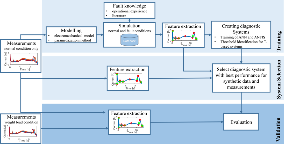
Figure 1 - Concept of the analysis
2. Disconnector Fundamentals: Components and Faults
Air insulated disconnector’s main function is to create an electrical connection or a separation between electrical circuits. They cannot switch load currents and but create a visible disconnection. This allows safe working on downstream electrical equipment [16]. Fig. 2 shows the basic structure of a pantograph disconnector. It consists of a frame (1) holding the support insulator (2). The support insulator is necessary as it carries the gear box (3) which is connected electrically and mechanically to the disconnector arms (4) and is thus at high-voltage potential. The mechanical force is generated by a DC-motor (5), transmitted by the rotary insulator (6) and converted in the gear box into an up and down movement of the disconnector arms. The arms must exert sufficient contact pressure to the contact point (7) to ensure a good electrical connection [17]. A bad electrical connection could thermally overload the disconnector during operation resulting in damages of the arms or the counter contact of the power line.
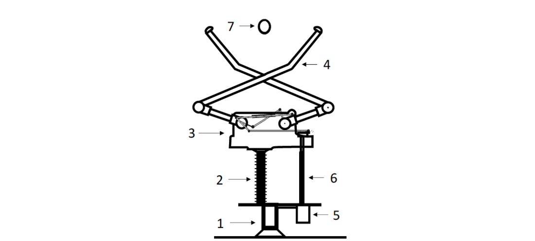
Figure 2 - Structure of a pantograph disconnector
Various events or processes lead to major failures of air-insulated high-voltage disconnectors with 0.29 major failures per 100 years per disconnector. The frequency of these failures increases with the equipment ageing [18]. The failures can be traced back to four main failure modes [19].
- Current path: Increased resistance due to worn or corroded contacts,
- Kinematic chain: Reduced material strength due to cracks of cast parts of the disconnector or corrosion. This finally leads to braking of mechanical parts.
- Drive: Corrosion due to water ingress into drive casing. Corrosion leads to gearbox sluggishness or even a blocked motor.
- Electrical control and auxiliary circuit: Corrosion leads to bad connections at the auxiliary switches and other electrical components. Increased moisture also causes short circuits of auxiliary contacts.
70.4 % of the disconnector major failures result in not closing or opening and 6.7 % result in locking in the open or closed position [20]. Fig. 3 shows the origin of major failures of 1,493 reported failures. The most major failures (34.8%) occur due to failures in the mechanical operating mechanism.
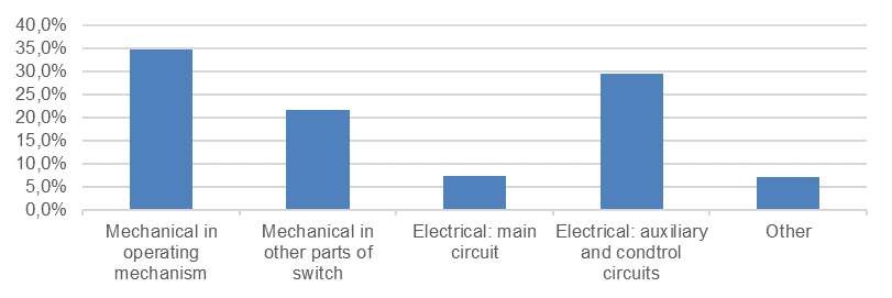
Figure 3 - Origin of major failures of disconnectors [20]
The design of pantograph disconnectors influences their reliability. Undersized mechanical joints may result in faults in the kinematic chain due to material failure. Insufficiently sealed components, either due to design flaws or due to material failure of sealings, may result in corroded metal parts or in damaged electrical components. Harsh weather conditions such as high salt content in the air may accelerate these ageing processes.
3. Diagnostic System and Modelling
In this paper, three diagnostic methods are developed using with synthetic data. The diagnostic systems are based on adaptive neuro-fuzzy interference systems (ANFISs), artificial neural networks (ANNs) and simple thresholds (Ts). ANFISs are based on fuzzy logic. Fuzzy logic transforms a feature space into fuzzy sets. Rules and membership functions imitate the continuous reasoning of humans [21] and can be used for diagnostic purposes [22], [23]. ANFIS utilises neural learning methods to optimize parameters and the structure of Fuzzy Interference Systems [24]. ANNs can be used as a nonstatistical-based data-driven fault diagnosis tool and are well-established [25]–[27]. The input of the diagnostic systems comprises features extracted from continuous-time signals.
3.1. Generation of Synthetic Data Using Normal- and Fault-Conditions Simulations
Often, only limited normal-condition measurements and no fault-condition measurements are available. To circumvent this problem, synthetic data can be generated using an electromechanical model. In measurements, a variation of the measured variables can be observed due to external or internal influences. These influences are often only partially represented in a model, as models typically simplify the cause-effect relationships. It follows that the variation of the model output does not match that of measurements. It is important that ML-based diagnostic systems are trained with synthetic data that reproduce the variation of measurements for robustness. Therefore, the simulation needs to account for the variation in normal conditions into account that is not covered by the electromechanical model. Furthermore, ML-based diagnostic systems need to be trained with fault-condition data. As fault-condition measurements are often not accessible, a fault-condition simulation needs to be implemented to generate training data for supervised ML. The fault condition simulation also needs to account for the variation that is not covered by the electromechanical model.
The simulation method consists of three core components: an electromechanical model of the equipment, an algorithm for parameter optimisation of the electromechanical model and the generation of parameter combinations of the electromechanical model. With the parameter optimisation algorithm, the electromechanical model can be fitted to measurement data to minimise the error between model output and measurements. With this algorithm and the available measurements, a database of the parameters of the electromechanical model is created by fitting the electromechanical model multiple times to different measurements. From this parameter database, another algorithm generates parameter combinations for normal and fault conditions. With these parameters, the electromechanical model is parameterised and simulated. Synthetic data can thus be generated.
The simulation of the variation within the normal condition requires normal-condition measurements of the monitored value or values to determine model parameters. An optimisation of m model parameters is conducted to minimise the error between the measurement and the model’s output. This results in n parameter sets of ?1,…,? for the model. Each set contains m parameters of ?1,…,?. These parameter values are used to calculate probability distributions for each parameter and to fit a normal distribution, as shown in Fig. 4 a). When a normal-condition simulation is conducted, the parameter values of the electromechanical model are randomly selected according to the probability distribution of each parameter [28]–[31].
For fault-condition simulation, it is necessary that fault conditions with a low intensity or pre-fault conditions are simulated. This is because large deviations from the normal condition can be identified using statistical or unsupervised learning methods. For fault conditions with low intensity and pre-fault conditions, it is assumed that the physical model is valid. For the simulation, it is not possible to derive parameter distributions from measurements, as often no fault-condition measurements are available. The fault-condition simulation creates new probability distributions of selected parameters in regard to the previously derived parameter distributions of the normal condition. The idea behind this is that if parameters are selected outside of the established normal-condition distribution, a simulation with such a parameter should result in an abnormal condition [28]–[31]. In Fig. 4 a) an abnormal probability distribution is illustrated. The probability distribution ranges from ?????????? ?????????+5 ? to ?????????? ?????????+25 ?, where s is the standard deviation of the normal condition’s normal distribution.
However, an abnormal condition is not necessarily a fault condition. For this purpose, a fault definition FD, measured in the standard deviation s, is introduced. Three fault definitions are shown in Fig. 4 b). If one of the model parameter values exceeds the fault definition, the simulation is considered as a fault-condition simulation. If no parameter value exceeds the fault definition, the simulation is considered as a normal condition. Different fault definitions are introduced in order to train diagnostic systems with different sensitivities [28].
The introduced abnormal probability distribution ensures existence of normal-condition data with a fault intensity close to the fault definition. Depending on the parameter value and the fault definition, the generated synthetic data are labelled as a normal condition or a fault condition.
The proposed method is not capable of simulating drastic fault conditions resulting in a completely changed equipment behaviour. Only faults or failure modes that can be linked to parameters of the electromechanical model can be simulated.
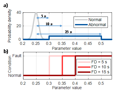
Figure 4 - (a) Normal- and abnormal-condition distribution of the motor friction parameter [28] / (b) Fault definitions [28]
3.2. Feature Extraction
To derive significant input data for the ML models, features are extracted from raw signals. These features are the input for the diagnostic system. They represent physical events in the monitored process or can be the result of mathematical operations. Features can represent a variety of measurement values, such as mean, mean square, standard deviation and integrals, as well as local minima or maxima from the time domain, the derivative or the frequency domain.
3.3. Concept of the ML-Based Diagnostic Systems
ML models can be used as classifiers. To that end, ML models automatically learn rules from given training data. The training data contain labelled data such as ‘normal condition’ and e.g. ‘fault type 1’. It is common to not provide raw signals as input data for the ML models but extracted features from the signals. For the diagnostic system, one model per simulated fault type is trained. The training data are labelled such that only the data of the specific fault type is labelled as faulty, the rest is interpreted as ‘normal condition’. The model is trained with the labelled data. After a successful training, the ML model is capable to predict whether unseen data or extracted features belong to ‘normal condition’ or ‘fault condition’ on a scale ranging from 0 to 1.
The structure of the complete diagnostic systems is shown in Fig. 5 and is divided into four parts: data pre-processing, ML models, condition detection and fault classification. In the pre-processing, features are extracted from the data. The ML model part contains one ML model for each analysed fault type. Every ML model outputs one value ???1…?. The outputs are combined to generate the diagnostic systems’ output for fault detection as follows. If the output ???1…? of any of the ML models is greater than a threshold q, the diagnostic system’s output is ‘fault condition’. If a fault condition is detected, the diagnostic system checks which ML model’s output ???1…? is the greatest. The fault corresponding to this particular ML model is the output of the fault classification system.
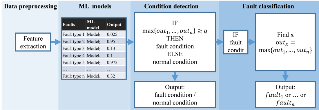
Figure 5 - Concept of the ML-based diagnostic systems
3.4. Threshold System (T)
The advantage of the T-based systems is that they are quickly parameterized and the results are comprehensible. The T-based system checks whether any feature ?? exceeds a predefined threshold value b, as shown in (1)[1]. is the output for each check and
and
are the upper and lower thresholds. The output of the T-based system is determined by (2). If desirable, the thresholds can be adjusted for sensitivity as per (3) and (4). ?? 0 is the initial threshold for the upper value and ?? 0 the initial threshold for the lower value. X is a factor for increasing (X > 1) or for decreasing (X < 1) the threshold band.
(1)
(2)
(3)
(4)
The T-based diagnostic system only detects but does not classify fault types. For a fault type classification, a knowledge management system would be necessary.
[1] Note that the threshold for ML systems q is different from the T-based system threshold b.
3.5. Metric to Evaluate the Diagnostic System’s Performance
Every ‘fault’ diagnosis can lead to expensive inspection or maintenance. Therefore, it is important to pay special attention to the true negative diagnoses (equipment is in normal condition and the diagnostic system has the output ‘normal condition’). The weighted condition detection rate ????? calculates the detection rate of a system by weighting the diagnoses of the normal condition with a factor of a. The WCDR is calculated using (13), where CD is the number of correct diagnoses and n the number of normal conditions or fault conditions in the data set. The higher a, the bigger the impact of true negative diagnoses on the WCDR is. Therefore, a should be chosen by the equipment owner considering the individual inspection and maintenance planning.
(13)
4. Results for a Pantograph Disconnector
The diagnostic systems for the pantograph disconnector detect faults by analysing the motor current of the drive motor, as power consumption analysis is well suited for fault detection and diagnosis [32]. Multiple ANFIS- and ANN-based diagnostic systems with varying hyperparameters are trained with synthetic data with three different fault definitions FD. The generated diagnostic systems are broadly analysed by examining the WCDR for normal-condition measurements and synthetic data. The aim of this analysis is to select the optimal diagnostic systems for detecting faults of a pantograph disconnector using only the synthetic data and available normal condition measurements. The selected diagnostic systems are then tested using measurements from a pantograph disconnector with additional weight load to check if ML-diagnostic systems trained with synthetic data are valid
predictors for real-world applications.
4.1. Experimental Setup: Measurements in Normal and Fault Condition
The validation of the diagnostic systems, requires real measurements. For this purpose, experiments with a 245 kV pantograph disconnector are carried out. The disconnector is switched multiple times and the current of the DC drive motor is measured. The pantograph disconnector has to create an electrical connection with the above located counter contact fixed to the busbar, even if the height of the busbar has changed e.g. due to a change in ambient temperature (see Fig. 6) The position of the counter contact has a large influence on the contact force and energy that has to be provided by a drive. This variation is respected in the experimental setup by varying the relative distance from the middle of the contact point of the disconnector to the busbar between -230 mm and +230 mm (see Fig. 6). The ambient temperature is kept in a range between 4°C and 8.8°C. With this setup, 61 measurements of a disconnector in normal condition during a making process are be obtained for further analysis.
As real fault-condition measurements are not available, the pantograph disconnector is loaded with additional weight. Adding weights to the arms of the disconnector imitate e.g. icing of the disconnector’s arms, strong corrosion of the joints or some damages of the supporting spring (see Fig. 6). According to the utility experience, the icing of arms and of the counter contact have led to a major malfunction of the device in the past. Hence, this fault case is very relevant for the proper diagnostic. 4.5 kg, 13.6 kg, 18.1 kg, 22.6 kg are added sequentially to its arms (see Table VIII for the corresponding quantity of measurements). The disconnector is operated with the added weight and the DC drive motor current is measured.
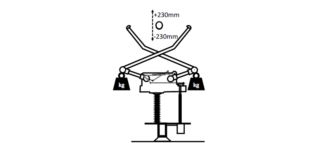
Figure 6 - Schematic of the experimental setup
4.2. Extracted Features
In the case of the disconnector’s motor current during a making process, 51 features are automatically extracted from the signals. Three classes of features (absolute features, gradient features and deviation features) are shown in Fig. 7.
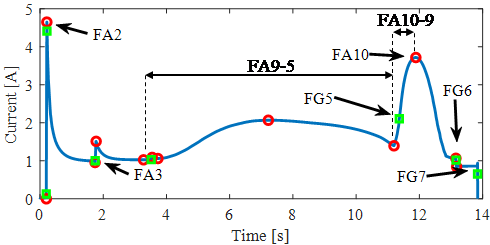
Figure 7 - Absolute (red) and gradient features (green) highlighted in the motor current signal. The features represent physical events in the disconnector’s closing process
| Feature | Event |
|---|---|
| FA1t, FA1I | Switching on the motor |
FA2t, FA2I | Inrush current of the motor |
FA3t, FA3I | No-load current with pre-resistor |
FA4t, FA4I | Current peak due to short-circuiting of the series resistor |
FA5t, FA5I | No-load current without pre-resistor |
FA6t ,FA6I | Mechanical connection between motor and swing arm |
FA7t, FA7I | Begin of the upward movement of the arms |
FA8t, FA8I | Current peak during upward motion |
FA9t, FA9I | Arm contacts counter contact |
FA10t, FA10I | Maximal pressure against counter contact |
FA11t, FA11I | Re-activation of pre-resistor (maximum) |
FA12t, FA12I | Re-activation of pre-resistor (minimum) |
FA13t, FA13I | Switching off the motor (maximum) |
FA14t, FA14I | Switching off the motor (minimum) |
| Feature | Event |
|---|---|
FG1t, FG1I | Switching on the motor: maximal positive gradient |
FG2t, FG2I | Inrush current of the motor: maximal negative gradient |
FG3t, FG3I | No-load current with pre-resistor: maximal positive gradient |
FG4t, FG4I | Mechanical connection between motor and swing arm: maximal positive gradient |
FG5t, FG5I | Buildup of contact force: maximal positive gradient |
FG6t, FG6I | Re-activation of pre-resistor: maximal negative gradient |
FG7t, FG7I | Switching off the motor: maximal negative gradient |
4.3. Setup of the Experiment: Method for Training and Evaluation of the Diagnostic Systems
Synthetic normal- and fault-condition training data are generated using the model of a pantograph disconnector. The model is taken from the literature and implemented in MATLAB Simulink [17]. The probability distributions of the parameters for the simulation are identified using the 61 normal-condition measurements of the disconnector’s motor current. The synthetic normal-condition data are verified by means of available normal-condition measurements.
Seven physical and electrical faults, listed in Table III, are simulated. The faults are based on the operational knowledge of utility personnel. For this paper, the parameter distributions for simulating abnormal conditions are uniform and range from 5 s to 25 s (Fig. 4 a). A starting point of 5 s ensures that the parameter to simulate the fault condition is selected outside of the established normal-condition distribution. Such a starting point results in fault conditions that match theoretical fault analysis [28]. In total, 20,000 simulations are carried out in eight groups, each containing 2,500 simulations. One group contains normal-condition data, where the normal distribution of the parameter is assumed. The other seven groups contain the synthetic data simulated with the abnormal conditions from Table III.
| Fault | Model parameter |
|---|---|
Short circuit or deformation of the drive motor windings | Factor for motor magnetisation function |
Short circuit of the drive motor windings, increased cable resistance | Motor resistance value |
Increased friction in the drive motor | Coefficient of friction |
Increased friction in the disconnector arm joints | Coefficient of friction |
Changed elasticity in the arm | Spring constant |
Inconstant supply voltage | Voltage |
Damaged drive motor current pre-resistor (reduced resistance or shorted) | Resistance |
In the next step, the main discrete features are extracted from every generated synthetic signal. The ANFIS- [24] and ANN-based [33] systems are trained with the features extracted from the 20 000 synthetic normal- and fault-condition data. The task is to classify if the data belongs to a fault condition or a normal condition. For the training, the simulations are divided into 80% training data and 20% validation data for the training of the ANN- and ANFIS-based diagnostic systems to avoid overfitting.
To find a diagnostic system with the greatest performance or correct diagnosis rate, numerous ANFIS [24] and ANN models [33] are trained with different hyperparameters (see Table IV and Table V accordingly). All combinations of the hyperparameters are considered. ANNs with a linear node activation function act as a linear regression model.
| Parameter | Investigated values |
|---|---|
Training method | - BFGS quasi-Newton backpropagation |
Numbers of layers | - one layer |
Node activation function | - hyperbolic tangent sigmoid |
| Parameter | Investigated values |
|---|---|
Training method | - backpropagation |
Numbers of considered indicators | - three indicators |
Because the computing time for the ANFIS training is remarkably longer than that for the ANN training, a subset of the extracted features is used as ANFIS input. In order to find the most valuable features for each ANFIS model, a sensitivity analysis for all features and the hyperparameters listed in Table IV is conducted. Each training is repeated 24 times with the same configuration to minimize the possibility that the final result is a local minimum. To train diagnostic systems with different fault sensitivities, three fault-condition definitions (FD = 5 s, FD = 10 s, and FD = 15 s) are determined, as shown in Fig. 4 b).
The initial boundaries ??,?0 and ??,?0 of the T-based system are set for each feature to the minimal or the maximal feature value that appeared in the normal-condition simulations. The factor X is varied in the range of 0 to 4 in increments of 0.1. The trained diagnostic systems are analysed using the seven measurements from the disconnector loaded with additional weight.
4.4. Evaluation of the Synthetic Normal-Condition Data
To evaluate the synthetic normal-condition data, 2,500 normal-condition data are generated with the method described in section 3.1. The envelope of the synthetic normal-condition data and the measurements are shown in Fig. 8. Features are extracted from the measurements and the synthetic data. The probability distributions of the features extracted from the synthetic data are compared to the features of the measurements. This is to verify that the synthetic data model the measurement sufficiently accurate. The boxplots of representative extracted features, normalized to the mean of each feature of the measurements, are shown in Fig. 9. The percental deviation of characteristic values of the synthetic data’s boxplots to the corresponding boxplot values of the measurements are shown in Table VI. The feature ??8? , time of the local maximum during the upward movement, has the largest deviation. The upper whisker of the synthetic data deviates by 31.96% from the upper whisker of the measurements. As Fig. 8 shows, the modelled upward movement between 5 s and 11 s does not show a distinct local maximum as the measurements do. This results in big variations of ??8? . The upper whisker of ??10? , the current peak during the build-up of the contact force, has a deviation of 26.67 % from the measurements whereas the lower whisker has a deviation of 0.01 % only. The mean of all the deviations of the characteristic boxplot values is 5.57 % and the median of all features deviates by an average of 6.25 %. This shows that the simulation is capable of modelling most of the distribution of the features sufficiently accurate.
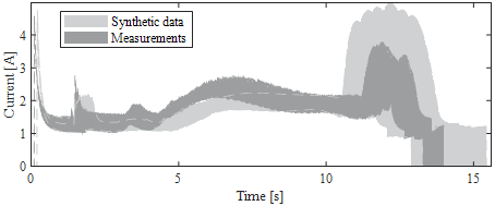
Figure 8 - Envelopes of the synthetic data and the measurements [28]
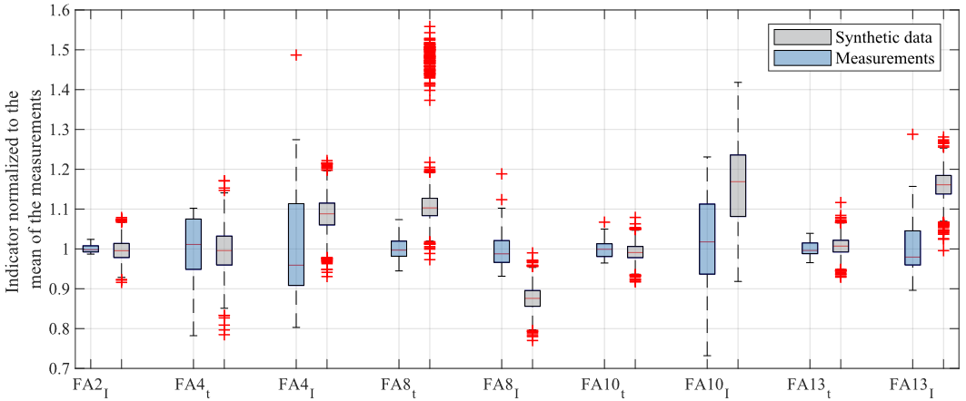
Figure 9 - Boxplots of selected features of the synthetic data and measurements. The data are normalized to the mean indicator value of the measurements
| Deviation from the measurements [%] | |||||
|---|---|---|---|---|---|
Lower whisker | 25th-percentile | Median | 75th-percentile | Upper whisker | |
FA2I | -13,66 | -3,89 | -0,85 | 1,37 | 9,68 |
FA4t | 1,85 | 1,78 | 0,87 | 0,51 | 13,36 |
FA4I | 2,74 | 9,95 | 11,01 | 0,11 | 1,14 |
FA8t | 2,98 | 12,29 | 16,03 | 20,48 | 31,96 |
FA8I | -22,92 | -11,86 | -10,83 | -7,85 | -2,50 |
FA10t | -5,01 | 1,00 | 2,91 | 5,94 | 13,94 |
FA10I | 0,01 | 11,31 | 13,92 | 12,33 | 26,67 |
FA13t | -4,30 | 1,69 | 4,78 | 7,47 | 17,35 |
FA13I | 14,06 | 17,39 | 18,41 | 14,45 | 12,45 |
4.5. Evaluation of the ML Models
Fig. 10 a) shows the histogram of the output of the considered ANN models applied to the simulated data. 99.7% of the ANN models converge either to one (fault condition) or to zero (normal condition), with a tolerance of 0.02. Therefore, the fault threshold ???? of Fig. 10 can be set to any value between 0.02 and 0.98, and no further investigation in finding an optimal threshold value is needed. For the following evaluation, ???? is set to 0.5.
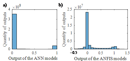
Figure 10 - (a) Histogram of the ANN models’ output -(b) Histogram of the ANFIS models’ output
Fig. 10 b) shows a histogram of the output of all ANFIS-based models for all simulated data. 92.1% of the outputs are in the range between –0.5 and 1.5. The ANFIS models do not converge to certain values. The threshold ?????? needs to be adjusted in order to find the optimal fault thresholds. Therefore, ?????? is variated in the range of –0.1 to 1.1 in increments of 0.1.
4.6. General Performance Evaluation of the Diagnostic Systems
Multiple diagnostic systems with different hyperparameters are build. In a real-world application, only could be implemented to detect faults. Therefore, a selection of a diagnostic system needs to be conducted without using the measurements of the disconnector loaded with additional weight. The diagnostic systems are evaluated against measurements in different data sets:
- measurements consisting of normal conditions only, as fault-condition measurements are not available
- simulated normal conditions
- simulated fault conditions.
The results of all considered diagnostic systems (different hyperparameters such as training methods, number of nodes, etc.) with a fault definition of ?? = {5 s, 10 s, 15 s} are presented in Fig. 11, Fig. 12 and Fig. 13. The fault intensity increases with an increase in fault definition. The selection of the best diagnostic system is a two-criteria optimisation problem that is evaluated with Pareto frontiers (thick line). Systems of the Pareto frontier describe the solution where no other system improves one criterion without diminishing another criterion. A ????20 is used to evaluate the diagnostic systems for the simulated data. ????1 represents the rate of correct diagnosis for measurements where the weighting factor has no influence.
Table VII lists the characteristic information of the Pareto frontiers for the considered diagnostic systems:
- the Pareto frontier tuple with the highest ????? (HW)
- the area under the Pareto frontier (AuF) (see also Fig 11.).
This characteristic information allows a comparison of different Pareto frontiers. The AuF characterises the whole frontier whereas the HW characterises the optimal point regarding one criterion. An AuF value close to 1 indicates the Pareto frontier of a system with good performance.
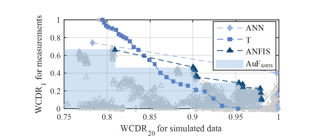
Figure 11 - WCDR of the diagnostic systems for a fault definition of ?? = 5 ?.
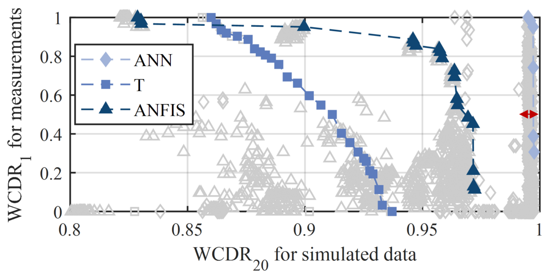
Figure 12 - WCDR of the diagnostic systems for a fault definition of ?? = 10 ?.
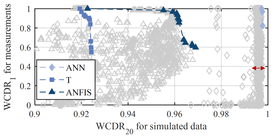
Figure 13 - WCDR of the diagnostic systems for a fault definition of ?? = 15 ?.
For a fault definition of ?? = 5 ? the Pareto frontiers of the T-based systems are superior to the ANN- and ANFIS-based systems. The T-based systems have a smaller HW for the simulations than the ANFIS- and ANN-based systems, but there are T-based systems that always classify the measurements correctly, leading to the largest AuF ( ??? = 0.86 ) of the three methods. The results show that the ANN-based systems are superior to the ANFIS- and T-based systems for a fault definition of FD = 10 s and FD = 15 s, with AuFs of 0.966 and 0.998, respectively. For these fault definitions, there are T-, ANFIS- and ANN-based systems that always classify the conditions of the measurements correctly.
The Pareto frontier systems of the ANN- and ANFIS-based systems show good validation results for the normal-condition measurements, with a ????1 of up to 100% for ?? = 15 ?. However, there are ANN-based systems with good results for the simulated data where the validation for measurements shows comparably poor results (clustered in a ????20 range between 99.1% and 99.8%, highlighted with a red arrow). This indicates that ANFIS- and ANN-based systems trained with simulated data also need to be validated with measurements.
An overall improvement in the Pareto frontiers with an increasing fault definition can be observed. This indicates that the transferability of the Pareto frontier systems trained with simulated data to measurements is better with a fault definition FD = 15 s. The ANN-based frontier systems outperform the T- and ANFIS-based ones. Therefore, ANN-based systems, trained with synthetic data with a fault definition FD = 15 s and a high WCDR for measurements and simulated data should be chosen for the real application.
| FD | T | ANFIS | ANN | |
|---|---|---|---|---|
5 s | HW for simulations | (0.953 | 0) | (0.980 | 0.097) | (0.999 | 0) |
HW for measurements | (0.794 | 1) | (0.783 | 0.742) | (0.809 | 0.661) | |
AuF | 0,857 | 0,600 | 0,668 | |
10 s | HW for simulations | (0.937 | 0) | (0.972 | 0.11) | (0.998 | 1) |
HW for measurements | (0.860 | 1) | (0.828 | 1) | (0.995 | 1) | |
AuF | 0,904 | 0,955 | 0,997 | |
15 s | HW for simulations | (0.919 | 1) | (0.923 | 1) | (0.997 | 1) |
HW for measurements | (0.924 | 0.548) | (0.969 | 0.597) | (0.998 | 0.823) | |
AuF | 0,924 | 0,966 | 0,998 |
4.7. Validation of Selected Diagnostic Systems
In section 4.6, it is shown that the ANN-based systems, trained with synthetic data with a fault definition FD = 15 s is most suitable for the real application.
Therefore, these diagnostic systems are evaluated for seven measurements of the disconnector loaded with additional weight. Because the systems are not trained to identify this additional weight load, the evaluation validates whether the diagnosis output is plausible or not. The evaluation checks whether 1) all seven measurements of additionally loaded disconnector are diagnosed as normal conditions (insensitive), 2) the rate of fault-condition diagnosis increases with increasing weight (plausible), or 3) the rate of fault-condition diagnosis is unrelated to the weight (implausible).
Fig. 14 shows a detail of the results of the ANN-based systems trained with ?? = 15 ? and a high WCDR for both synthetic data and measurements. The ANN-based systems are marked according to whether they are implausible, plausible or insensitive. The figure shows, that none of the ANN-based systems trained with ?? = 15 ? and a high WCDR for synthetic data and measurements show implausible diagnosis for the data of the disconnector loaded with additional weight. This indicates that utilizing MLdiagnostic systems for real applications is possible.
The diagnostic system with the highest ????20 for the synthetic data is insensitive to weights. Therefore, the diagnostic systems, S1 and S2 showing plausible classification results for the data of an additionally loaded disconnector are further evaluated. Table VIII presents the detection rate for the systems S1 and S2 (marked in Fig. 14) for the measurements from the disconnector loaded with additional weight. Both systems are trained with a Levenberg–Marquardt algorithm and have one layer with seven (System S1) and eight (System S2) nodes and a hyperbolic tangent sigmoid transfer function. System S1 diagnoses all data sets with weights ≥ 18.1 kg as fault conditions; System S2 diagnoses all data sets with weights ≥ 13.6 kg as fault conditions.
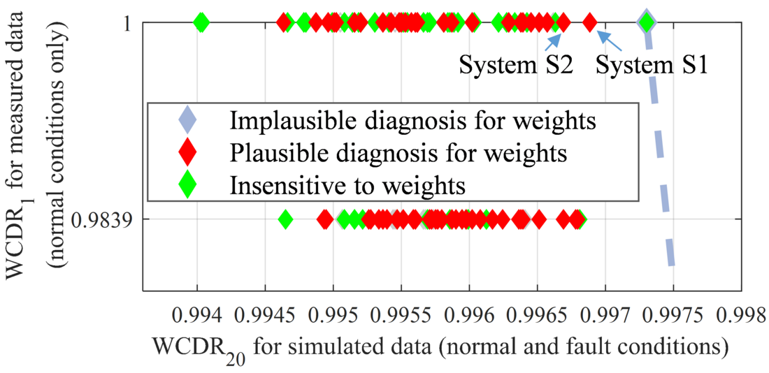
Figure 14 - Diagnosis of additional weights on the disconnector arms for systems trained with ?? = 15 ?
| Diagnosis: Fault condition | ||||
|---|---|---|---|---|
Weight [kg] | 4,5 | 13,6 | 18,1 | 22,6 |
Quantity of data sets | 1 | 2 | 1 | 3 |
System S1 | 0% | 0% | 100% | 100% |
System S2 | 0% | 100% | 100% | 100% |
Additionally, the remaining ANN- and ANFIS-based diagnostic systems are tested with the measurements from the disconnector loaded with additional weight. In total, 65.7% of the ANN-based systems trained with ??=15 ? are plausible, 15.0% are insensitive, and 19.3% are implausible systems for weights attached to the disconnector arms. For the ANFIS-based systems, 92.2% of the systems are plausible, 7.7% are implausible, and 0% are insensitive when applied to the measurements from the disconnector loaded with additional weight.
From the previous analysis we can conclude that transferring ML-based diagnostic systems to real-world application is possible and even detect fault conditions they are not trained for.
5. Conclusion
In this paper, it is examined whether synthetic data can be used to generate diagnostic systems for real-world application when fault-condition measurements are not available. ANN- and ANFIS-based diagnostic systems trained with synthetic data and T-based diagnostic systems were considered. The synthetic data were generated with an electromechanical model of a disconnector and a normal-condition and a fault-condition simulation method. Different fault intensities were considered in the process. A multi-criteria verification and validation was conducted on the rate of correct diagnoses for measurements and simulated data to identify potential diagnostic systems for real-world application. The multi-criteria evaluation prevented selecting overfitted of ANN and ANFIS models, models that always predicting the normal conditions for measurements. The evaluation shows that the rate of correct diagnosis for synthetic data depends on the fault type, the fault intensity, the ML algorithm and the algorithm hyperparameters.
The ANN-based diagnostic systems with a high WCDR for both synthetic data and measurements are the most appropriate for the pantograph disconnector. These diagnostic systems are validated against measurements from a disconnector with additional weight load to imitate a fault that the diagnostic systems are not trained with. Even though the diagnostic systems are not trained for that specific use case, 65.7% of the ANN-based diagnostic systems and 92.2% of the ANFIS-based ones were capable of plausibly detecting the modification.
The investigation shows that ML-based diagnostic systems trained with synthetic data are promising and it could be applied to other equipment and applications. Further research is needed to validate the proposed method for other applications.
References
- Ewg, Energiewirtschaftsgesetz: Gesetz über die Elektrizitäts- und Gasversorgung EnWG. Letzte Änderung 18/12/2018., 2005.
- Y. Han und Y. H. Song, “Condition monitoring techniques for electrical equipment - a literature survey”, IEEE Trans. Power Delivery, 18. Jg., Nr. 1, pp. 4–13, 2003.
- H. Su und K. T. Chong, “Induction Machine Condition Monitoring Using Neural Network Modeling”, IEEE Trans. Ind. Electron., 54. Jg., Nr. 1, pp. 241–249, 2007.
- M. Zekveld und G. P. Hancke, “Vibration Condition Monitoring using Machine Learning” in IECON 2018 - 44th Annual Conference of the IEEE Industrial Electronics Society, 2018.
- S. Ma, M. Chen, J. Wu, Y. Wang, B. Jia und Y. Jiang, “High-Voltage Circuit Breaker Fault Diagnosis Using a Hybrid Feature Transformation Approach Based on Random Forest and Stacked Autoencoder”, IEEE Trans. Ind. Electron., 66. Jg., Nr. 12, pp. 9777–9788, 2019.
- T. Boukra, A. Lebaroud und G. Clerc, “Statistical and Neural-Network Approaches for the Classification of Induction Machine Faults Using the Ambiguity Plane Representation”, IEEE Trans. Ind. Electron., 60. Jg., Nr. 9, pp. 4034–4042, 2013.
- K.-C. Park, Y. Motai und J. R. Yoon, “Acoustic Fault Detection Technique for High-Power Insulators”, IEEE Trans. Ind. Electron., 64. Jg., Nr. 12, pp. 9699–9708, 2017.
- A. Singh und P. Verma, “A review of intelligent diagnostic methods for condition assessment of insulation system in power transformers” in 2008 International Conference on Condition Monitoring and Diagnosis: IEEE, 2008, pp. 1354–1357.
- M. Dumitrescu, T. Munteanu, D. Floricau und A. P. Ulmeanu, “A Complex Fault-Tolerant Power System Simulation” in 2005 2nd International Conference on Electrical and Electronics Engineering: IEEE, Sep. 2005, pp. 267–272.
- R. Gitzel, I. Amihai und M. S. Garcia Perez, “Towards Robust ML-Algorithms for the Condition Monitoring of Switchgear” in 2019 First International Conference on Societal Automation (SA), Piscataway, NJ, USA: IEEE, 2019, pp. 1–4.
- Z. Meng, X. Guo, Z. Pan, D. Sun und S. Liu, “Data Segmentation and Augmentation Methods Based on Raw Data Using Deep Neural Networks Approach for Rotating Machinery Fault Diagnosis”, IEEE Access, 7. Jg., pp. 79510–79522, 2019.
- Y. Wu, C. Lu, G. Wang, X. Peng, T. Liu und Y. Zhao, “Partial Discharge Data Augmentation of High Voltage Cables based on the Variable Noise Superposition and Generative Adversarial Network” in 2018 International Conference on Power System Technology (POWERCON), Piscataway, NJ, USA: IEEE, 2018, pp. 3855–3859.
- S. Afzal, M. Maqsood, F. Nazir, U. Khan, F. Aadil, K. M. Awan, I. Mehmood und O.-Y. Song, “A Data Augmentation-Based Framework to Handle Class Imbalance Problem for Alzheimer’s Stage Detection”, IEEE Access, 7. Jg., pp. 115528–115539, 2019.
- A. Ypma, Learning methods for machine vibration analysis and health, Ph.D. dissertation, Delft, Netherlands, 2001.
- X. Li, W. Zhang, Q. Ding und J.-Q. Sun, “Intelligent rotating machinery fault diagnosis based on deep learning using data augmentation”, J Intell Manuf, 31. Jg., Nr. 2, pp. 433–452, 2020.
- Handbuch Elektrotechnik: Grundlagen und Anwendungen für Elektrotechniker ; mit 300 Tabellen, 5. Aufl., Wiesbaden, Vieweg+Teubner Verlag / GWV Fachverlage GmbH Wiesbaden, 2009.
- B. Rusek, C. Neumann und N. Lambrecht, “Monitoring and Diagnosis of Pantograph Disconnectors” in Internationaler ETG-Kongress, Vorträge des internationalen ETG-Kongresses, J. W. Kreusel, Ed., Berlin, Germany: VDE-Verl., 2009.
- M. Runde, C. E. Sölver, A. Carvalho, M. L. Cormenzana, H. Furuta, W. Grieshaber, A. Hyrczak, D. Kopejtkova, J. G. Krone, M. Kudoke, D. Makareinis, J. F. Martins, K. Mestrovic, I. Ohno, J. Östlund, K.-Y. Park, J. Patel, C. Protze, J. Schmid, J. E. Skog, B. Sweeney und F. Waite, “Final Report of the 2004 - 2007 International Enquiry on Reliability of High Voltage Equipment: Part 1 - Summary and General Matters, Working Group A3.06”, Nr. 509, 2012.
- A. Maheswari, B. Rusek, B. Sweeney, C. Fischer, D. Makareinis, L. Gauthier, L. O'Sullivan, N. Amyot, P. Del Crego Amo, T. Minagawa und T. Lindquist, “Ageing High Voltage Substation Equipment and Possible Mitigation Techniques: Working Group A3.29, Technical Brochure”, Nr. 725, 2018.
- M. Runde, C. E. Sölver, A. Carvalho, M. L. Cormenzana, H. Furuta, W. Grieshaber, A. Hyrczak, D. Kopejtkova, J. G. Krone, M. Kudoke, D. Makareinis, J. F. Martins, K. Mestrovic, I. Ohno, J. Östlund, K.-Y. Park, J. Patel, C. Protze, J. Schmid, J. E. Skog, B. Sweeney und F. Waite, “Final Report of the 2004 - 2007 International Enquiry on Reliability of High Voltage Equipment: Part 3 – Disconnectors and Earthing Switches, Working Group A3.06”, Nr. 511, 2012.
- Z. Gao, C. Cecati und S. Ding, “A Survey of Fault Diagnosis and Fault-Tolerant Techniques Part II: Fault Diagnosis with Knowledge-Based and Hybrid/Active Approaches”, IEEE Trans. Ind. Electron., pp. 1, 2015.
- S. Simani, S. Farsoni und P. Castaldi, “Fault Diagnosis of a Wind Turbine Benchmark via Identified Fuzzy Models”, IEEE Trans. Ind. Electron., 62. Jg., Nr. 6, pp. 3775–3782, 2015.
- Q. T. Tran, S. D. Nguyen und T.-I. Seo, “Algorithm for Estimating Online Bearing Fault Upon the Ability to Extract Meaningful Information From Big Data of Intelligent Structures”, IEEE Trans. Ind. Electron., 66. Jg., Nr. 5, pp. 3804–3813, 2019.
- A. T. Azar, “Adaptive Neuro-Fuzzy Systems” in Fuzzy Systems, A. Taher, Ed., Rijeka, Croatia: InTech, 2010, pp. 85–110.
- Y. Shatnawi und M. Al-khassaweneh, “Fault Diagnosis in Internal Combustion Engines Using Extension Neural Network”, IEEE Trans. Ind. Electron., 61. Jg., Nr. 3, pp. 1434–1443, 2014.
- S. Toma, L. Capocchi und G.-A. Capolino, “Wound-Rotor Induction Generator Inter-Turn Short-Circuits Diagnosis Using a New Digital Neural Network”, IEEE Trans. Ind. Electron., 60. Jg., Nr. 9, pp. 4043–4052, 2013.
- H. C. Cho, J. Knowles, M. S. Fadali und K. S. Lee, “Fault Detection and Isolation of Induction Motors Using Recurrent Neural Networks and Dynamic Bayesian Modeling”, IEEE Trans. Contr. Syst. Technol., 18. Jg., Nr. 2, pp. 430–437, 2010.
- J. N. Kahlen, A. Mühlbeier, M. Andres, B. Rusek, D. Unger und K. Kleinekorte, “Electrical Equipment Analysis and Diagnostics: Methods for Model Parameterization, Fault and Normal Condition Simulation” in Proceedings of International Conference on Condition Monitoring, Diagnosis and Maintenance, Sep. 2019, pp. 43–52.
- J. N. Kahlen, A. Würde, M. Andres und A. Moser, “Model-based Data Augmentation to Improve the Performance of Machine-Learning Diagnostic Systems” in Proceedings of the 22nd International Symposium on High Voltage Engineering, Cham: Springer International Publishing, 2021.
- J. N. Kahlen, M. Andres und A. Moser, “Improving Machine-Learning Diagnostics with Model-Based Data Augmentation Showcased for a Transformer Fault”, Energies, 14. Jg., Nr. 20, pp. 6816, 2021.
- J. N. Kahlen, A. Würde, M. Andres und A. Moser, “Improving Machine Learning Diagnostic Systems with Model-Based Data Augmentation - Part A: Data Generation” in 2021 IEEE PES Innovative Smart Grid Technologies Europe (ISGT-Europe): IEEE, Oct. 2021.
- A. H. Sabry, F. H. Nordin, A. H. Sabry und M. Z. Abidin Ab Kadir, “Fault Detection and Diagnosis of Industrial Robot Based on Power Consumption Modeling”, IEEE Trans. Ind. Electron., 67. Jg., Nr. 9, pp. 7929–7940, 2020.
- S. S. Haykin, Neural networks and learning machines, 3. Aufl., New York, Pearson, 2009.
Biographies

Dr. Jannis Nikolas Kahlen was born in Freising, Germany, in 1992. He received his B.Sc., M.Sc., and Ph.D. in electrical engineering in 2014, 2016, and 2021 from RWTH Aachen University, Aachen, Germany. He works as a Research Associate at the Institute for High Voltage Equipment and Grids, Digitalization and Power Economics, RWTH Aachen University, and the Fraunhofer Institute for Applied Information Technology. His research focuses on data analysis, artificial intelligence, simulation and modelling for diagnostics and asset management in the field of electromechanical devices.

Artur Mühlbeier was born in Almaty, Kazakhstan, in 1987. He received the B.Sc. and M.Sc. degrees in electrical engineering from RWTH Aachen University in 2010 and 2013 respectively. From 2013 to 2019, he has been a research assistant at the Institute for High Voltage Technology of RWTH Aachen University. Since 2020, he is with BatterieIngenieure GmbH in Aachen, Germany.

Dr. Michael Andres, received his Diploma Degrees in Electrical Engineering (2011) as well as “Business Administration & Engineering” (2012) from RWTH Aachen University (Germany). From then on he worked in different leading positions for the Institute of High Voltage Technology. Michael received his doctorate in Engineering (2016) from the RWTH Aachen University gaining knowledge on analysis and modelling of oil-filled distribution transformers in normal and overload operation. Since 2017, Michael leads the department “Digital Energy” in the Fraunhofer-Institute of Applied Information Technology (FIT). The department offers interdisciplinary expertise from “Designing Future Energy Supply Systems” up to “IT Security Technologies”.

Dr. Bartosz Rusek received his M.Sc. from TU Wroclaw in Poland and his PhD from TU Darmstadt in Germany both in electrical engineering. Since 2006 he works for a German transmission system operator Amprion GmbH in the department of asset management. He was involved the topics of EHV equipment maintenance, renewal strategies, life cycle models, asset data management systems, dynamic line rating and insulation coordination of HV AC/DC hybrid lines. He is responsible for integration of new innovative technologies into EHV grid. He contributes in different working groups and steering committees in FNN, DKE, CIGRE, Entso-E.

Dr. Dennis Unger was born in Lünen, Germany, in 1985. He received his diploma degree in electrical engineering and management in 2009 and his Ph.D. in electrical engineering in 2016, from TU Dortmund University, Dortmund, Germany. From 2015 to 2019 he worked in the asset management department at Amprion GmbH, Dortmund, Germany. Since 2020 he is head of the department Asset Management at Dortmunder Energie- und Wasserversorgung GmbH, Dortmund, Germany.

Dr. Klaus Kleinekorte received a diploma in electrical engineering and a PhD degree from the University of Technology Aachen. Since 1992 he worked with RWE in various management functions. In October 2003 he was appointed to the Board of today’s Amprion GmbH. As CTO his main area of responsibility comprised Asset Management/Grid Planning and the Control Centre Brauweiler. As Chairman of the UCTE Working Group Operations and Security Mr. Kleinekorte was strongly involved in the development of the UCTE Operation Handbook. He was member of the ENTSO-E Assembly. Within CIGRE he represented Germany at the Administration Council and the Steering Committee.