A new partial discharge measuring system in HVGIS based on magnetic field antennas
Authors
A. RODRIGO-MOR, F. MUÑOZ- MUÑOZ, L. C. CASTRO-HEREDIA, A. NAYAK
Delft University of Technology, The Netherlands

Summary
For more than 45 years, Gas Insulated Switchgear (GIS) has been in operation, showing high reliability and low failure rates. Recently, the introduction of DC systems in the offshore application has brought the HVDC GIS as the most suitable technology because of its aforementioned high reliability. Nevertheless, the experience from the field has shown that some in-service failures may occur, in which many of these defects are related to the insulation system. For this reason, partial discharge detection systems play an essential role in the monitoring and diagnostic of HV GIS (GIS) due to its high capabilities to detect in-service failures related to defects in the insulation system.
This paper presents a new measuring system for partial discharges in gas-insulated systems (GIS). The measuring system is based on magnetic antennas tuned at the high-frequency range, in which the PD pulse travels according to the transmission line theory. The measuring system consists of three magnetic antennas deployed in a GIS, current amplifiers, a high-speed acquisition system, and a post-processing technique to estimate the apparent charge and source location. The magnetic antenna characterization, the measuring system sensitivity, charge estimation and localization capabilities are studied. Laboratory experiments were conducted in a 380 kV GIS at the High Voltage Laboratory of Delft University of Technology, where corona discharges under DC voltage were created in two different GIS compartments. The results demonstrate the suitability of the measuring system for PD detection in GIS, charge estimation and source location. Under laboratory conditions, the antenna sensitivity is in the order of 5 pC at a few meters from the PD source.
Keywords
Partial discharges - GIS - magnetic antenna - charge estimation - partial discharge localization - sensitivity check1. Introduction
The ultra-high frequency (UHF) method is the most extensively partial discharge measuring system used in GIS systems because it is less influenced by noise, which is mainly concentrated at low frequencies [1]. The UHF method is based on capacitive couplers, tuned at the ultra-high frequency range (300 MHz to 3 GHz), that are installed in the enclosure dielectric windows. This method has the advantage that the GIS enclosure acts as a Faraday cage, shielding the UHF sensors from external electromagnetic interferences, allowing a low background noise level, and resulting in high sensitivity. Its high sensitivity and high resilience to EMI has consolidated its application as a standard for on-line monitoring in AC GIS, resulting in a solid practice that is being transferred to HVDC GIS.
However, the UHF method captures the electric field signals produced by the PD activity in the high-frequency range, where the electromagnetic waves suffer significant attenuation and distortion, causing that the sensitivity of the PD detection substantially decays with the distance between the partial discharges (PD) source and the sensor [2–8]. Additionally, in the UHF range is not possible the apparent charge estimation in pC because of the high electromagnetic wave distortion due to the complex propagation characteristics at high frequency. On the other hand, at low frequencies (kHz – hundreds of MHz), a PD pulse travels according to the transmission line theory. Therefore, the current is distributed based on the characteristic impedance, resulting in less attenuation and distortion. When a PD is triggered, it creates a surface current that travels along the inner part of the compartments and the outer part of the main conductor.
Therefore, the PD detection in GIS faces two scenarios: a high-frequency one which is less affected by the noise, but with high attenuation and distortion, and another –at low frequency- with less attenuation and distortion but strongly influenced by the noise coming from inverter control or power supply systems. Keeping this in mind and considering the advances in post-processing techniques and measurement technologies, we have developed a new PD measurement system for GIS. This new measuring system relies on a magnetic antenna that measures the PD current at the low-frequency range, where this magnetic-detection approach boosts the spatial sensitivity by seizing the lower attenuation of the low-frequency spectrum of the PD signals with distance. Also, this system aims to make progress towards improving the location of the PD source and reducing the effect of noise.
2. Fundamentals
In principle, in the GIS enclosure, a PD pulse produces a homogeneous surface current at the low frequencies due to its coaxial structure, as is presented in Figure 1. However, when the surface current reaches the dielectric windows, it loses its homogeneity and travels around the window. This deviation around the dielectric window produces a magnetic field normal to the dielectric window surface. This PD current has a transient behaviour causing a time-varying magnetic field. Figure 2 shows that this magnetic field induces an electric field in the dielectric window surface. Therefore, if a conductive closed loop is placed in the dielectric window, it will eventually have an induced voltage caused by the PD pulse travelling in the GIS compartments. This hypothesis has been proven and tested in [9,10].
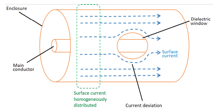
Figure 1 - Surface current distribution in the GIS enclosure
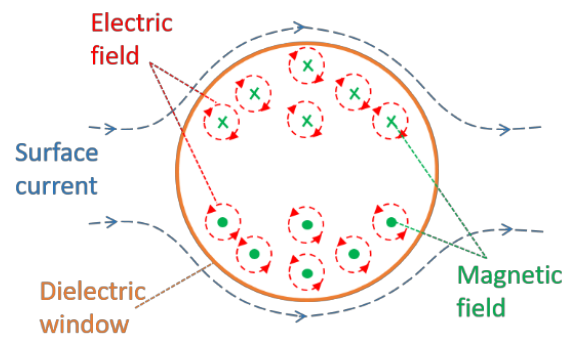
Figure 2 - Magnetic field and induced electric field in the dielectric window [9]
3. Magnetic antenna characterization
The magnetic antenna is made up of two shielded loops, as is presented in Figure 3. The loops were built in a half-circle shape using the coaxial cable RG179, which results in 218 nH inductance and 32 pF capacitance per loop. As is shown in Figure 3, a conductive mounting plate was added to the antenna to keep the internal Faraday cage capabilities of the GIS enclosure.
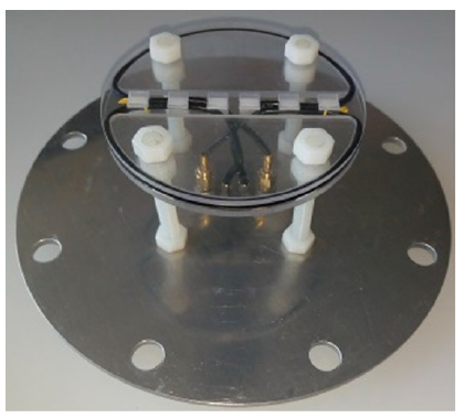
Figure 3 - Magnetic antenna[10]
The magnetic antenna is meant to be placed in the existing dielectric windows of the GIS enclosure, where the distance between the loops and the mounting plate is such that the antenna perimeter levels the edge of the internal wall of the dielectric window with the internal GIS enclosure. A 2 mm clearance between the loops diameter and the inner walls of the dielectric window has been chosen because it is necessary for the antenna installation to overcome the internal bump produced by the perimeter welding of the window pipe to the GIS compartment. The antenna diameter is 103 mm and the distance to the mounting plate is 53 mm.
Ideally, the magnetic antenna loops (named as top and bottom loop) measures only the magnetic field produced by the PD current in the enclosure, but it also measures the electric field produced by the PD pulse. The outer loop formed by the coaxial cable screen is only grounded in one side and left floating in the other to prevent short-loop currents and to provide electric field shielding. The inner loop formed by the inner coaxial cable conductor forms the measuring loop and is connected to a parallel of 2 x 0.055 μF decoupling capacitors and a commercial transimpedance amplifier model Femto HCA-40M-100K-C. The decoupling capacitor was added to block the DC feedback loop between the amplifier and the magnetic antenna. The schematic circuit is presented in Figure 4, where La1i represents the inner conductor inductance, La1o the screen inductance, Cca1 is the loop capacitance due to the coaxial cable, Cpa1 is the parasitic capacitance of floating end screen, Lh1 is the inductance of the hole in the GIS dielectric window, and K1, K2, and K3 are the coupling coefficients. Lh1 and the coupling coefficients have been calculated using electromagnetic finite element simulations.
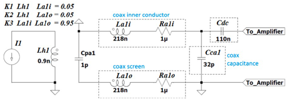
Figure 4 - Magnetic antenna equivalent electric circuit [10]
A test bench, specially designed for calibration purposes, was built to test the frequency response of the magnetic antenna and its associated components (decoupling capacitor + transimpedance amplifier). Figure 5 presents the test bench, which was equipped with two cones for matching the impedance of the GIS enclosure, avoiding reflections, and allowing the injection of high-frequency currents. The test bench consists of three GIS compartments, a wire (1 mm diameter) as the main conductor, and the injection and termination cones. The input current flowing through the main conductor was measured using a HFCT, model FCT-016-5.0 from Bergoz with 3.92 kHz–1.11 GHz bandwidth.
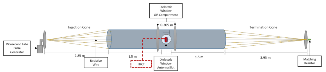
Figure 5 - Test bench
Figure 6 presents the input current in the time and frequency domain measured by the HFCT. The current pulse is a high-frequency and unipolar pulse injected with a pulse generator at the injection cone. The termination cone is not perfectly matched, causing small reflections of the current pulses, which interact with the unipolar-pulse distorting the frequency response. For this reason, the main conductor was made with resistive wire that attenuates the reflections, causing a clear and unique current pulse.
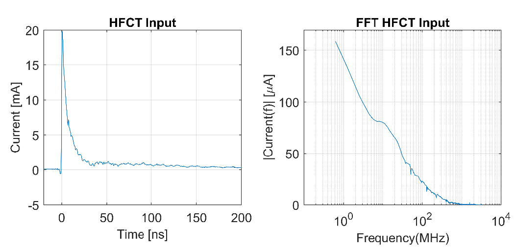
Figure 6 - Input current pulse
Figure 7 shows the output signal measured by one of the antenna loops. The frequency response of the magnetic antenna is presented in Figure 9.
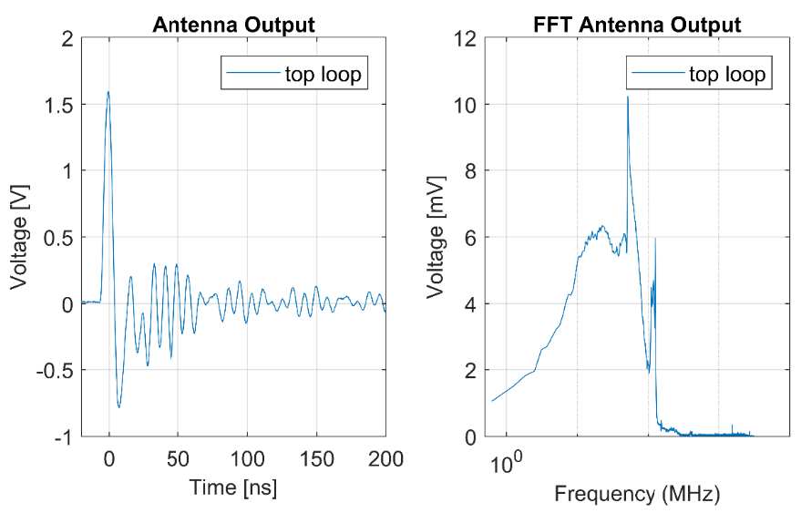
Figure 7 - Magnetic antenna output signal
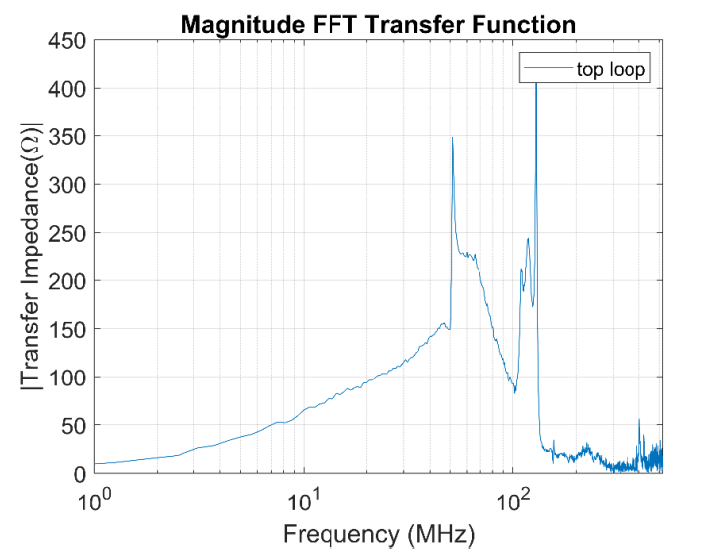
Figure 8 - Magnetic antenna frequency response
Some remarks about the magnetic antenna are given as follows:
- The frequency peaks are around 52 MHz and 125 MHz.
- The magnetic antenna is tuned at the High Frequency (HF) range, in opposition to the VHF and UHF ranges of the traditional electric antennas. This frequency range corresponds to the TEM propagation mode.
4. PD Measuring system in GIS
4.1. Test setup
A set of three magnetic antennas were tested in a 380 kV AC GIS at the High Voltage Laboratory of Delft University of Technology, where the SF6 was removed from all the GIS compartments. The GIS in Figure 9 consists of multiple spacers, a T-joint branch, switchgear, a bushing, an L-branch connection, a disconnector switch and eight dielectric windows for PD monitoring equipped with UHF antennas. Three UHF were removed and replaced by magnetic antennas at the locations highlighted in Figure 9. Two near the ends of the GIS and one in the middle point.
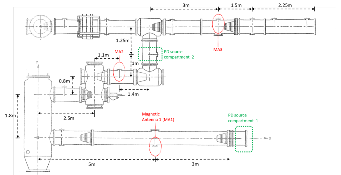
Figure 9 - GIS layout schematic
Inside the GIS, corona discharges were produced by two different sources, which were tested under DC negative voltage and separately (time-wise). The first corona source, named CS1, was built in a test cell under SF6 at 100 kPa (relative). Figure 10 shows the test cell installed in the GIS compartment 1, where a HFCT (FCT-016-5.0 Bergoz) was installed in the rod holding the CS1 to record the PD current at the source. A 25.5 dB amplifier was connected to the HFCT output to improve the signal to noise ratio. The HFCT at the source permits the charge estimation at the source, which will be useful for the evaluation of the charge estimation in section 4.4.
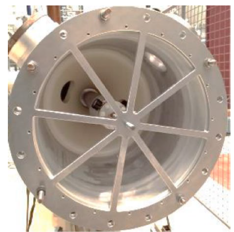
Figure 10 - Test cell at the GIS compartment 1 [10]
The second corona source, CS2, consisted of a needle connected at the main conductor in compartment 2. This defect was only monitored by the magnetic antennas, meaning that the HFCT was not connected. The purpose of the test with CS2 was to evaluate the magnetic antenna capabilities for PD localization.
The PD signals were recorded using the Tektronix MSO58 Fast Frame Acquisition Mode, which captures multiple PD pulses individually in a frame with a specific record length. The HFCT and the magnetic antennas were simultaneously sampled by the oscilloscope. Table 1 summarizes the different voltages and tests performed.
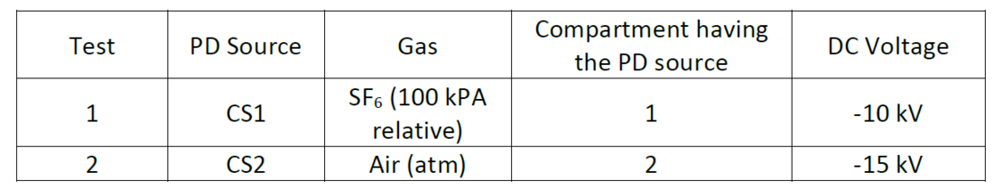
Table 1 - Test parameters
4.2. Results
This work uses a collection of 2 measurement results, which are used to verify the magnetic antenna performance. In total, the oscilloscope acquired 7000 PD signals, where 5000 PDs corresponded to test 1, and 2000 to the test 2. The PD charge estimation was only possible in Test 1 because it had the HFCT directly connected to the test cell. Figure 11 shows the apparent charge for the 5000 PD pulses collected in test 1, showing that the PD charge ranges between 4 pC and 170 pC. Figure 12 presents a characteristic PD pulse recorded by the magnetic antenna MA1 and the HFCT in test 1. The magnetic antenna signals show that the first peak of both loops appears around the same time (around 0.22 μs), the signals have different polarities and a pseudo-mirror-like symmetry. An ideal mirror-like symmetry cannot be obtained due to the noise and the manufacturing differences between both loops.
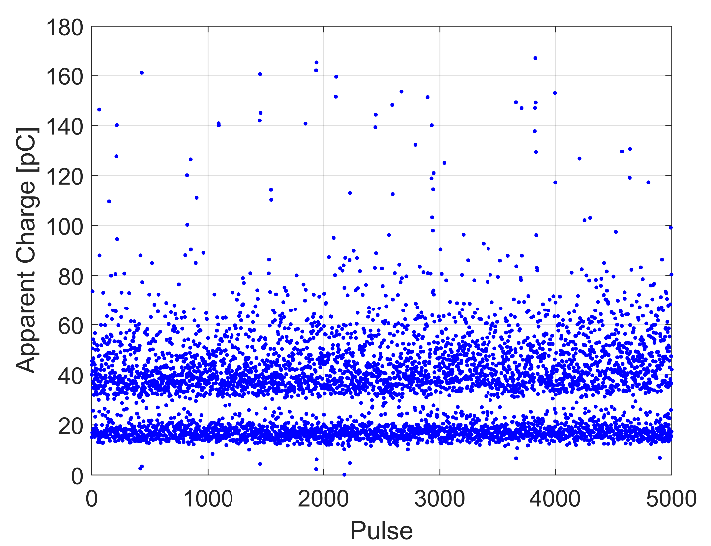
Figure 11 - The apparent charge for each of the PD pulses recorded in test 1
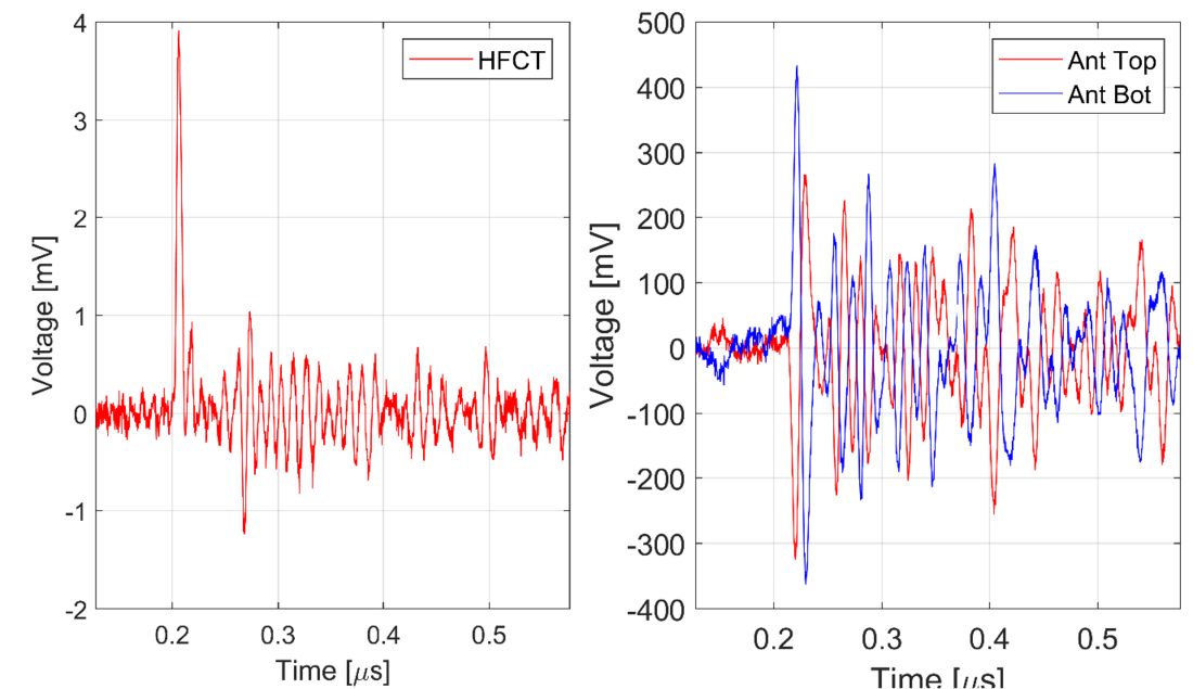
Figure 12 - PD pulse measured by the HFCT and the magnetic antenna MA1
4.3. Sensitivity
The magnetic antenna ability to detect PD pulses was tested using the results coming from test 1, where the apparent charge can be calculated. This ability to detect PD pulses was proven by checking the minimum charge detection level of the closest magnetic antenna to the test cell and the farthest one. The checking of the minimum detection level was done following three criteria: the peak amplitudes of both loops were synchronized, its peak magnitude was roughly two times the background noise, and its average power indicates a clear pulse.
The closest magnetic antenna to the test cell, MA1, was able to detect PD pulses having charges above 4.98 pC. Figure 13 shows the PD pulse recorded by the HFCT and the corresponding signals recorded by the magnetic antenna loops at the closest location. Both peaks occurred at the same time and the peak magnitudes are at least two times higher than the background noise. Regarding the average power, it shows two different zones: a flat zone at the beginning of the signal, followed by a significant rising of the power, where the flat zone corresponds to the background noise, and the increase of the power after the flat zone indicates the presence of the PD signal. On the other hand, the farthest antenna (MA3) could not detect this small PD, as is depicted in Figure 14. This is explained by the fact that the PD signals coming from the test cell split at the T branch, causing a reduction and distortion in the PD current flowing through the compartment where MA3 is installed.
Nevertheless, the farthest antenna to the test cell was able to detect PD pulses having charges above 15 pC. Figure 15 shows the PD pulse recorded by the HFCT and the signal recorded by the magnetic antenna loops at MA3.
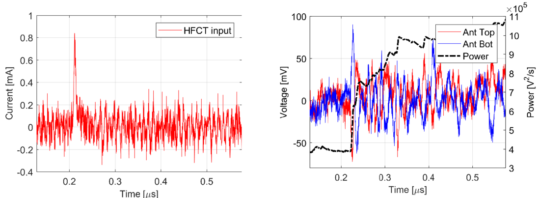
Figure 13 - PD pulse measured by the HFCT of the smallest PD pulse (4.98 pC) detected by MA1
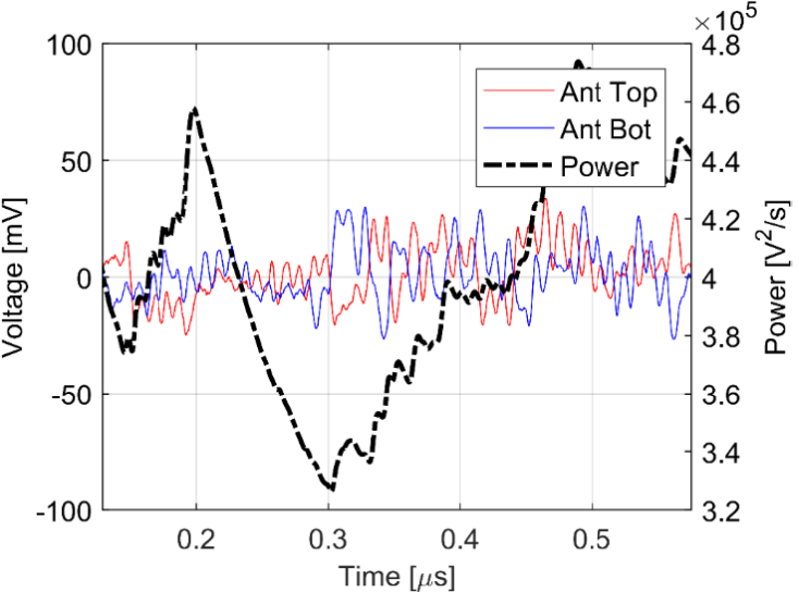
Figure 14 - Smallest PD pulse (4.98 pC) measured by MA3
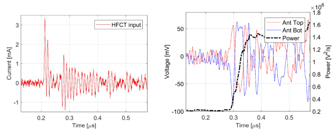
Figure 15 - PD pulse measured by the HFCT of the smallest PD pulse (15 pC) detected by MA3
4.4. Charge estimation
This section aims to analyse the possibilities for charge estimation of the PD signals that are produced in the test cell in the compartment 1 and that travel along the GIS reaching the magnetic antennas at position MA1, MA2 and MA3 in Figure 9.
For this purpose, the reference charge is calculated as the discrete integral of the current output of the Bergoz HFCT connected just next to the test cell. The signals from the HFCT are acquired with enough bandwidth and sufficient SNR such that the charge of the PD signal is estimated within an acceptable error.
Then, the charge estimation at different locations is studied as the comparison of the calculated value from the magnetic antenna and the reference charge value. Taking into account that the acquisition of all the channels of the oscilloscope is synchronous, then the estimated charge value of every signal from each antenna is 1-to-1 compared to the corresponding PD signal at the test cell that triggered the acquisition.
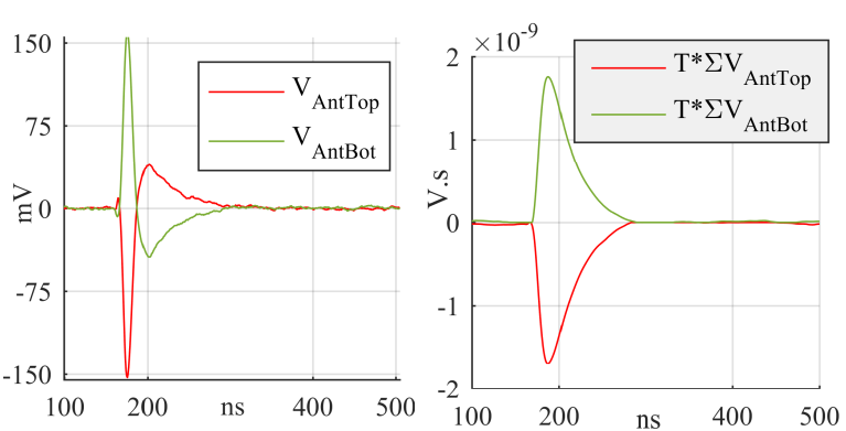
Figure 16 - Determination of the pseudo-current of the antenna’s output for charge estimation [10]
As reported in [10], the charge estimation from the antennas involves two steps before it can be correlated to the reference charge. The first step is the cumulative integration of the antenna’s voltage output as illustrated in Figure 16. This results in a pseudo-current signal that is then integrated to estimate the charge of the current in the vicinity of the coils of the antenna. The second step is to apply an experimental calibration factor [10] to calculate the charge equivalent to the total current flowing along with the GIS compartment. The experimental calibration factor was obtained by comparing the charge of known calibration pulses and the charge calculated from the antenna as per the aforementioned time-domain integration method.
Figure 17 shows the calibration rig having the same diameter as the GIS compartment. Using this set-up, the calibration factor was estimated as
Experimental results in the same GIS [10] showed that compensation of 1.3∙Kc adjusts better the reference charge and the charge estimated from the antenna’s output.
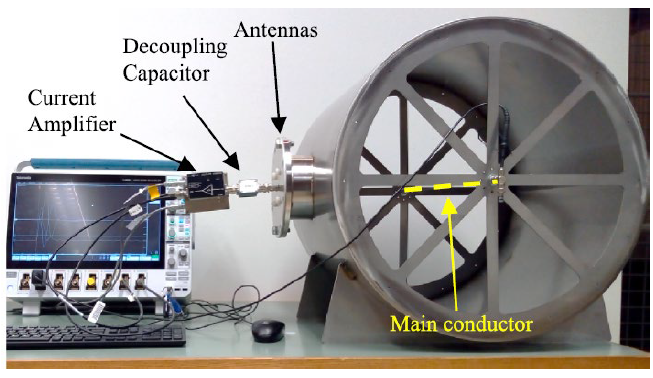
Figure 17 - Calibration rig set-up [10]
The results of the charge estimation are shown in Figure 18 with the colormap indicating bins of error compared to the reference charge. For the analysis of the charge estimation, only reference signals in the range from 10 to 30 pC were studied assuming that higher values of charge are not likely to be found in practice. Thus, plots in Figure 18 are populated with 1085 out of the total 5000 acquisitions.
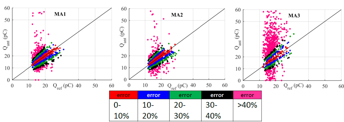
Figure 18 - Comparison of charge estimation at every location of the magnetic antenna
The charge estimation as per the time domain methods described above yielded to a varying error depending on two main factors: the distance to the PD source and the determination of the integration limits. For MA1 and MA2 most of the charge values fall into the 0-20 % error bins. This proves that after 3 m (MA1) and 14.2 m (MA2), the attenuation and distortion of the PD signals are still marginal despite already having travelled along with impedance changes such as the circuit breaker and the ground disconnector of the GIS. This resulted in very similar patterns for MA1 and MA2 plots. The larger scatter seen for MA3 was caused by the halving of the peak amplitude after the PD pulse splits into halves at the T-connector after compartment 2 (see Figure 9). The peak reduction is also a reduction of the SNR of the signal which strongly affects the correct determination of the integration limits. This situation is illustrated in Figure 19 top, where the output of MA1 and MA3 are shown corresponding to an input of 14.7 pC at the test cell. For the antenna MA1, the limits of the main peak of the cumulative integral were determined correctly by the algorithm thus leading to a charge estimation of 13.8 pC. However, due to the low peak amplitude of MA3, the limits are miscalculated resulting in an overestimation of the charge of 49.2 pC.
On the other hand, improvements of the algorithms to determine the integration limits will result in the reduction of the scatter of the charge estimation.
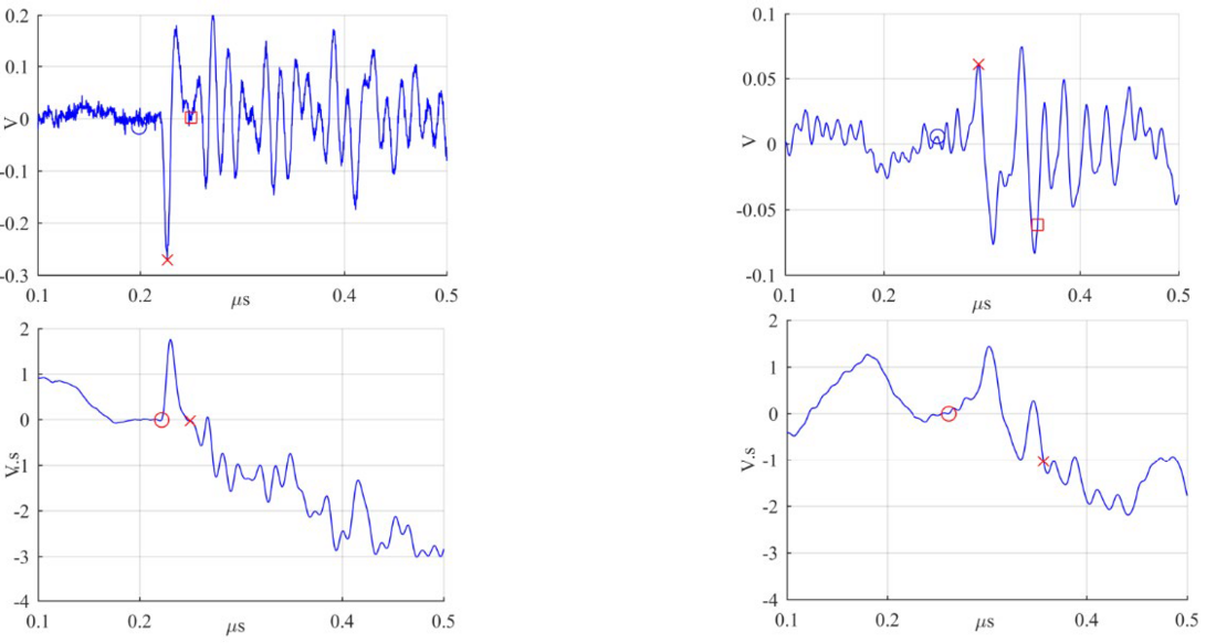
Figure 19 - Integration limits for MA1 and MA3 for a reference charge of 14.7pC shown in red dots. Tops: antenna’s output; Bottoms: cumulative integral of antenna’s output
4.5. Localization
This section gives some insights into the localization capabilities of the measuring system based on magnetic antennas. The localization capabilities are studied using the data collected during the test 2.
In test 2, the PD source was located at the compartment 2, which means that the PD source was at 2.4 m from the MA2, at 4.25 m from MA3, and at approx. 14 m from the MA1. Considering that the PD pulse travels along the GIS as in a transmission line, it is expected that MA2 first detects the PD signal, then MA3, and finally, the MA2.
Figure 20 corroborates this expectation, showing that the PD pulse is measured first by MA2, 5.7 ns later is detected by MA3, and 46.7 ns lately is measured by MA1; the peak value was used to determine the time of arrival.
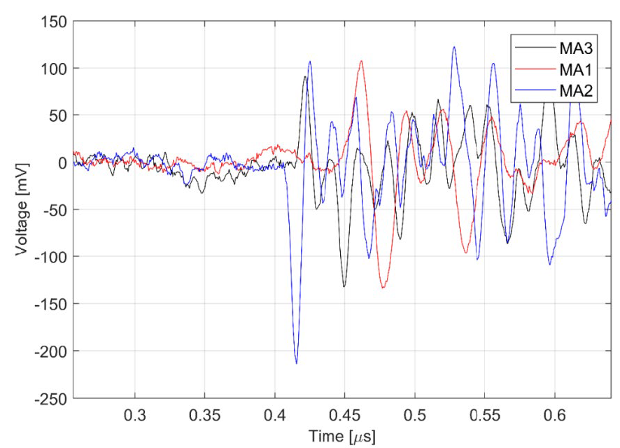
Figure 20 - PD pulse measured at MA1, MA2, and MA3, in which only one loop is depicted
Assuming that the speed of propagation is equal to the speed of light in vacuum, it is possible to estimate the distance between the defect and the magnetic antenna MA3 using equation (1).
(1)
Where Δt is the time difference between MA2 and MA3, c is the speed of light in vacuum, xT is the distance between the two antennas, and x is the distance between MA3 and the defect. Therefore, the estimated distance is:
(2)
It means that the distance between the PD source and the magnetic antenna MA3 is 4.18 m, which is relatively closer to the real value mentioned before (4.25 m). Now, using the MA1, MA2, and the MA3, the estimated distance between the magnetic antenna 1 and the PD source is:
(3)
In this case, the estimated distance between the magnetic antenna 1 and the defect is 12.60 [m], having an absolute error of 1.11 [m].
5. Conclusion
This paper shows that the measuring system based on magnetic antennas is a feasible option for partial discharge monitoring on HV GIS. The magnetic antenna frequency response indicates that the antenna is tuned in the HF range, in which the PD pulse travels according to the transmission line theory. The experimental results with corona discharges have shown that the magnetic antenna is able to detect small partial discharges, in the order of 5 pC at 3 m and 15 pC at 20.85 m distance from the PD source. Additionally, it has been possible to estimate the apparent charge of the partial discharges using the double integral method and the calibration factor proposed in [10]. For the closest antenna to the PD source, most of the estimated charge values fall into the 0-20 % error, but a larger error in the estimation was seen for the farthest antenna. It has been proven the localization capabilities of the measuring system, where the PD source was located using the arrival time between the antennas.
References
- Schichler, U.; Koltunowicz, W.; Gautschi, D.; Girodet, A.; Hama, H.; Juhre, K.; Lopez-Roldan, J.; Okabe, S.; Neuhold, S.; Neumann, C.; et al. UHF partial discharge detection system for GIS: Application guide for sensitivity verification: CIGRE WG D1.25. IEEE Trans. Dielectr. Electr. Insul. 2016, 23, 1313–1321.
- Hikita, M.; Ohtsuka, S.; Teshima, T.; Okabe, S.; Kaneko, S. Electromagnetic (EM) wave characteristics in GIS and measuring the EM wave leakage at the spacer aperture for partial discharge diagnosis. IEEE Trans. Dielectr. Electr. Insul. 2007, 14, 453–460.
- Bell, R.; Charlson, C.; Halliday, S.; Irwin, T.; Lopez-Roldan, J.; Nixon, J. High-Voltage On-Site Commissioning Tests for Gas-Insulated Substations Using UHF Partial Discharge Detection. IEEE Power Eng. Rev. 2002, 22, 61.
- Hikita, M.; Ohtsuka, S.; Hoshino, T.; Maruyama, S.; Ueta, G.; Okabe, S. Propagation properties of PD-induced electromagnetic wave in GIS model tank with T branch structure. IEEE Trans. Dielectr. Electr. Insul. 2011, 18, 256–263.
- Hikita, M.; Ohtsuka, S.; Okabe, S.; Wada, J.; Hoshino, T.; Maruyama, S. Influence of disconnecting part on propagation properties of PD-induced electromagnetic wave in model GIS. IEEE Trans. Dielectr. Electr. Insul. 2010, 17, 1731–1737.
- Ohtsuka, S.; Teshima, T.; Matsumoto, S.; Hikita, M. Relationship between PD-induced electromagnetic wave measured with UHF method and charge quantity obtained by PD current waveform in model GIS. In Proceedings of the 2006 IEEE Conference on Electrical Insulation and Dielectric Phenomena; IEEE, 2006; pp. 615–618.
- Hikita, M.; Ohtsuka, S.; Wada, J.; Okabe, S.; Hoshino, T.; Maruyama, S. Propagation properties of PD-induced electromagnetic wave in 66 kV GIS model tank with L branch structure. IEEE Trans. Dielectr. Electr. Insul. 2011, 18, 1678–1685.
- Hikita, M.; Ohtsuka, S.; Ueta, G.; Okabe, S.; Hoshino, T.; Maruyama, S. Influence of insulating spacer type on propagation properties of PD-induced electromagnetic wave in GIS. IEEE Trans. Dielectr. Electr. Insul. 2010, 17, 1642–1648.
- Rodrigo-Mor, A.; Muñoz, F.; Castro-Heredia, L. A Novel Antenna for Partial Discharge Measurements in GIS Based on Magnetic Field Detection. Sensors 2019, 19, 858.
- Rodrigo Mor, A.; Castro Heredia, L.C.; Muñoz, F.A. A magnetic loop antenna for partial discharge measurements on GIS. Int. J. Electr. Power Energy Syst. 2020, 115, 105514.