Dynamic Current Rating – Thermal Transient Response
Authors
E. OLSEN, F. BRYNEM - Nexans, Norway
M. HATLO - Unitech Power Systems, Norway

Summary
Dynamic loads in three-core power cables are a central aspect in several common use cases, such as wind power. Being able to predict the thermal response to a change in load current can lead to better optimized and more cost-effective cable solutions. Many of the peak-load cases could potentially be taken advantage of, given the ability to reliably predict the cable’s thermal transient response. That ability could allow for temporary and controlled overloads, without the risk of overheating the cable, by taking advantage of the significant thermal inertia of buried cables. However, the size and scale of submarine cable systems make it quite demanding to collect experimental and representative data to verify a thermal model.
This article presents the experimental results from testing conducted on a full-scale three-core XLPE submarine cable in a simulated but realistic environment. It includes a comparison between the measured data, prevailing standards’ theoretical predictions, a Finite Element Model simulation, and the predictions of a numerical algorithm made specifically for this as a proof-of-concept.
The test setup consisted of a specialized test container with a three-core XLPE submarine cable mounted in its centre. The container was spacious enough to have approximately one meter of free space between the container walls and the power cable in all radial directions. It was filled with wet sand, a typical seafloor soil type. The power cable and soil temperatures were monitored with 21 thermal probes. The setup was connected to a dual-mode power supply that had the ability to output up to approximately 1600 A alternating or direct current. The current was measured and logged continuously.
The simulations showed mixed results. The IEC and the proof-of-concept model had some inconsistencies compared to the measured data. Though despite that, the results intimate that predicting thermal transients in three-core power cables is possible using relatively simple methods. The finite element model showed a more accurate prediction of the temperature data, compared to the two aforementioned methods.
Keywords
Cable – Dynamic Rating – Thermal Transient Response – Overload Temperatures – IEC 60853-21. Introduction
The purpose of this research is twofold: To investigate how well the methods provided by IEC correspond with experimental data, and to explore other methods of calculating thermal transients in three-core submarine cables.
The specific objectives of the experiment were:
- Measure the thermal transient response of a buried three-core submarine cable
- Build a numerical model specifically designed to model buried three-core cables
- Compare predictions of the prevailing standards to the empirical data
- Compare predictions of the numerical model to the empirical data
Experimental data was collected by setting up a test environment with a full-scale cable mounted in a soil-filled container. The cable was equipped with thermocouples and connected to a power source. Both temperature and current were logged via software developed in LabVIEW.
The submarine cable was first subjected to a constant load for approximately 12 days, which was sufficient to achieve thermal equilibrium; this represented the preload. Once in steady state, the cable was subjected to a series of load steps, some of which had a current higher than what the cable is rated for in steady state. Once the load cycles were completed, the current was dropped to zero and the cooling period was logged as well. The preload, cycling and cooling combined into a dataset spanning approximately 22 days, with temperature and current logged every 10 seconds.
IEC 60853-2 provides a method for calculating single-step transients. This method was first extended to allow for several steps, then it was used to predict the conductor temperature with a varying load pattern.
A separate model was developed as a proof-of-concept, which attempts to solve the same problem numerically. The model divides the entire system into elements (like a low-resolution mesh), and then it calculates the heat loss due to flowing currents and the energy transferred between each element. The thermal energy transferred in each timestep is translated into a change in temperature. If an element gains energy during a timestep, its temperature will increase in proportion to its heat capacity (and vice versa).
2. Description of the test environment
The test environment was set up to simulate a real-life cable installation buried in seabed sand, saturated with water.
2.1. Test object
Three-core XLPE submarine power cable, 245 kV 3x1x1200 Al
2.2. Test setup
Test tank (20-feet container, inner measures: L=6.0 m, W=2.4 m, H=1.8 m)
Test object positioned in the centre
Filled with sand and saturated with water
2.3. Power Supply
Power source; three-phase AC, 0-1600 A with VARIAC voltage regulator, manually operated
2.4. Measurement and logging
Thermocouples (pt100-elements)
National Instruments thermocouple interface
LabVIEW application for logging and presentation of data (logging interval 10 sec.)
A total of 21 thermocouples were installed in the cable and the soil around it at the centre of the container. The thermocouples in the surrounding soil were mounted on wooden brackets in the horizontal and vertical planes, see Figure 1. See Appendix A for details of the thermocouples position.
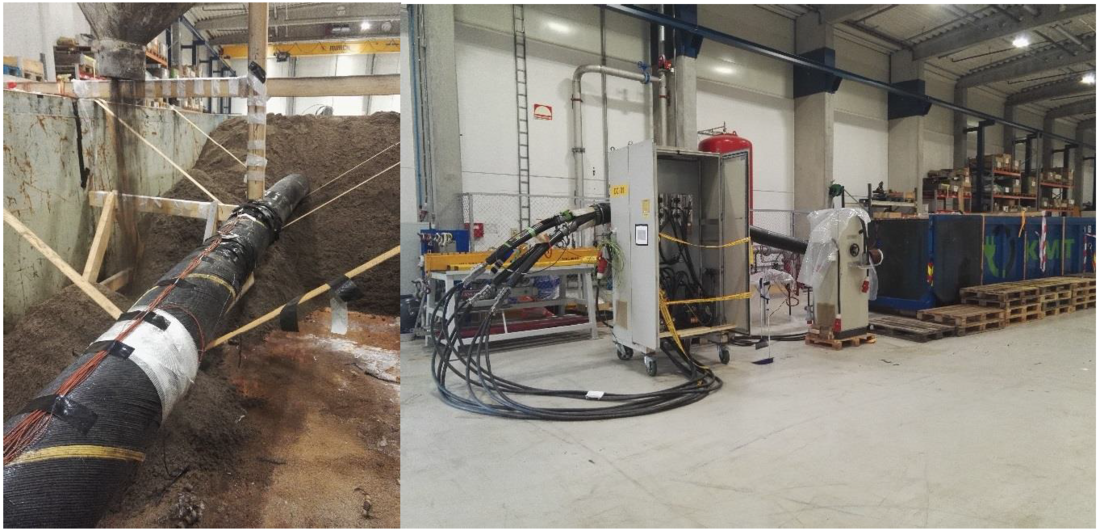
Figure 1 - Pictures of the test set-up
With all the thermocouples installed the container was filled with sand (fine-grained, typical seabed sand). The properties of the backfill material were obtained by measuring the thermal resistivity and moisture content in its different states. The results are presented in Table 1.
| Sample | Thermal resistivity [K.m/W] |
|---|---|
| Uncompacted, completely dried out | 1,65 |
| Uncompacted, saturated, (15,4 % moisture) | 0,42 |
| Compacted, completely dried out | 0,99 |
| Compacted, natural moisture (5,6 % moisture) | 0,40 |
| Compacted, saturated (5,9 % moisture) | 0,39 |
Afterwards the container was filled with tap water until a level where the sand-filling was completely covered (saturated). It is expected that the cables internals were completely flooded at that time.
For the conditions of the test container, the value for uncompacted and saturated (ρ = 0.42 K.m/W) was used in the simulations. In those conditions, the steady-state rating for the cable was found to be 1115 A (to reach a conductor temperature of 90 °C).
3. Thermal transient response
The principles adopted from IEC 60853-2 are shown in Figure 2. The idea is that the contribution from each change in load (load-step) gives a contribution to the total conductor temperature change, as shown in the figure.
This concept can be shown to be mathematically consistent with the heat equation in solids. The temperature at position r at time t, θ(r,t), inside the cable and its surroundings is described by the heat equation:
(1)
Where k(r) is the thermal conductivity, Cv(r) is the volumetric heat capacity, and Q(r,t) is the heat developed at position r (conductor, screen and armour) at time t. The general solution to the conductor temperature as a function of time can be written as a sum over all steps in heat development:
(2)
Where Gkl(t) is only a function of time, and ΔQc/s/a is the change in heat development in the conductor, screen and armour at time ti. A set of functions Gkl(t) exist for each position in the geometry, and may be estimated with analytical formulas, or numerically calculated with finite element software.
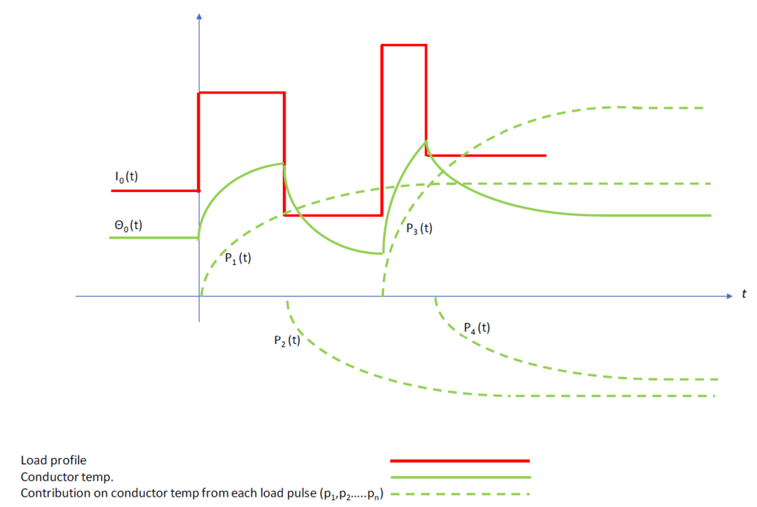
Figure 2 - Thermal transient response with varied current
This means that for every load-step, the contribution to the conductor temperature change is extended to infinity and that all pulses are superimposed continuously as the time elapses.
(3)
Since the methods in IEC 60853-2 is developed for a single load-step, an interpretation of the different models to achieve the total temperature response is necessary [1].
The conductor, screen, and armour losses are calculated according to a method similar to the one described in “Accurate analytical formula for calculation of losses in three-core submarine cables”, which has been validated by measurements on the same 245 kV 3x1x1200 Al cable [3], [4].
3.1. The IEC 60853-2 method
IEC 60853 gives a way to calculate the cable temperature as a function of time after a step in the load, and for several steps in the conductor current the equation for the conductor temperature is:
(4)
The losses in the screen and armour are embedded into the function G(t), which depends on the loss factors λ1 and λ2 in a nonlinear manner. This means that the solution as described by IEC is not consistent with the heat equation (1), for AC cables (λ1/λ2>0).
A general reference is made to IEC 60853-2 for details of the thermal transient response calculation [1].
3.2. Purpose-build model
The concept of the model is centred on dividing the system into a finite number of elements, as shown in Figure 3. Each element is associated with several thermal characteristics (resistance, capacity, temperature), as well as having interfaces to adjacent elements. Elements that are electrically relevant are equipped with an electrical overlay. The overlay feeds thermal energy into the system to simulate transmission losses.
Transient periods are divided into smaller increments, i.e. timesteps. The model assumes steady state conditions during each timestep. With that assumption, the energy exchange between elements is calculated in each timestep using steady state equations. That exchange of thermal energy translates into a change in temperature. Euler’s method is used to numerically calculate the energy exchange in each timestep.
The energy transfer in each time step is given by Fourier’s law, a simple first-order differential equation:
(5)
Where ΔT is the difference in temperature between two elements, and R is the thermal resistance.
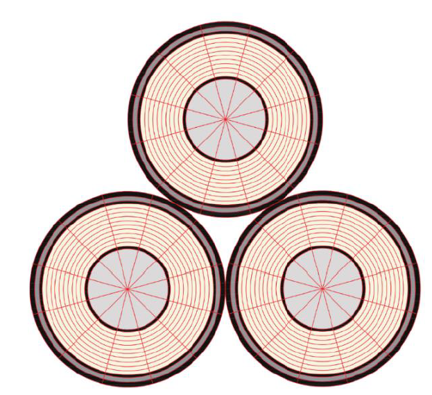
Figure 3 - Sketch of the mesh elements forming the cable’s thermal system
4. Results
4.1. Collected Data
Prior to application of the load sequence the system was run to a steady-state condition for a period of 12 days. The preload temperature equilibrium terminated at 67.3 °C for a current value of 937 A.
Then the following load sequence was applied:
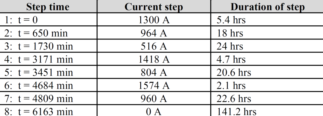
Table 2 - Applied load sequence at steady-state (t = 0)
The system’s thermal response to this load sequence is shown in Figure 4 and Figure 5. As expected, the conductor and the inner-most layers have a sharp and well-defined response to a sudden change in current. The outer-most layers and the external environment showed a dampened and delayed response. Note that the data also show a significant gradient across the armour layer; this is consistent with past research [2].
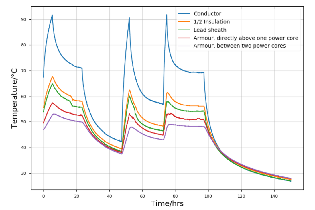
Figure 4 - Measured temperature in the cable internals
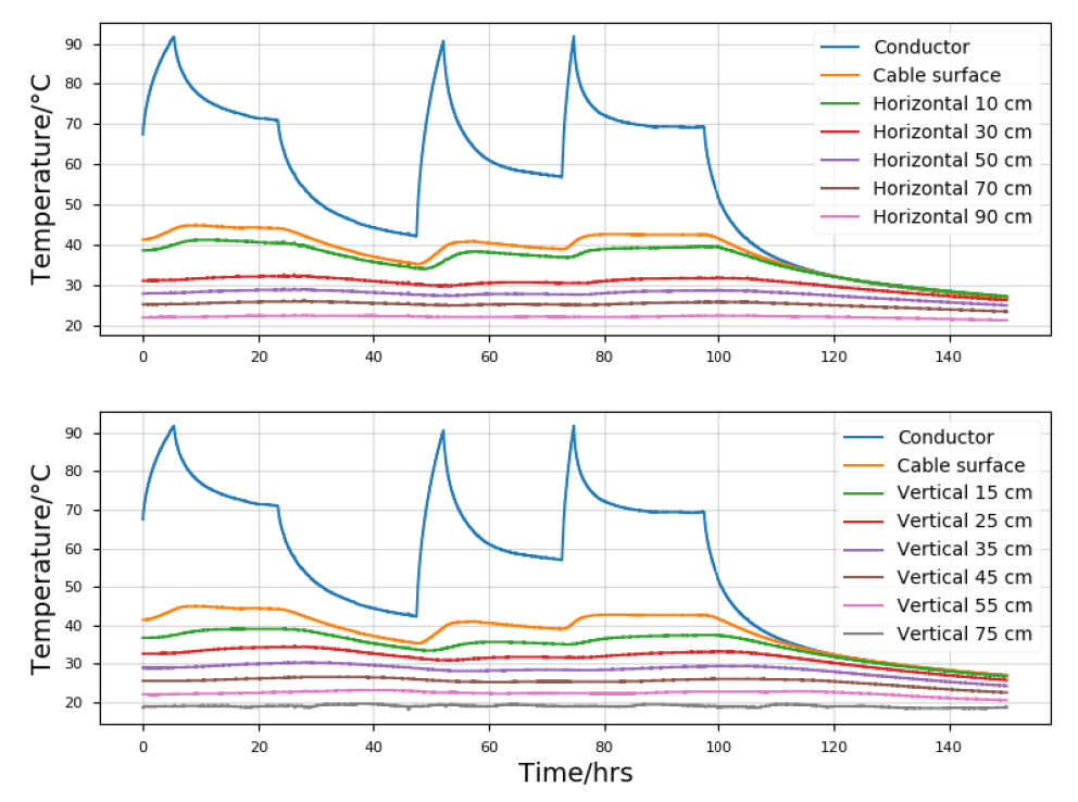
Figure 5 - Measured temperature from cable surface and outwards, with conductor temperature for reference
4.2. Comparison with IEC for the load sequence
The calculated and measured conductor temperatures for the load sequence are shown in Figure 6. The deviation at the first peak temperature is approximately 3 °C.
Since the test equipment comprised a manually fixed voltage variator, it was not possible to maintain a steady applied current throughout each load step; the current would drop as the conductor temperature and hence conductor resistance increased. To establish the load curve for the IEC simulation, the quadratic mean (r.m.s.) value of the measured current (10 sec. values) was used.
(6)
The values in Table 2 are established based on the measured current during each load step using the principles from Eq. (2) where n = total number of 10-sec. interval for each load step.
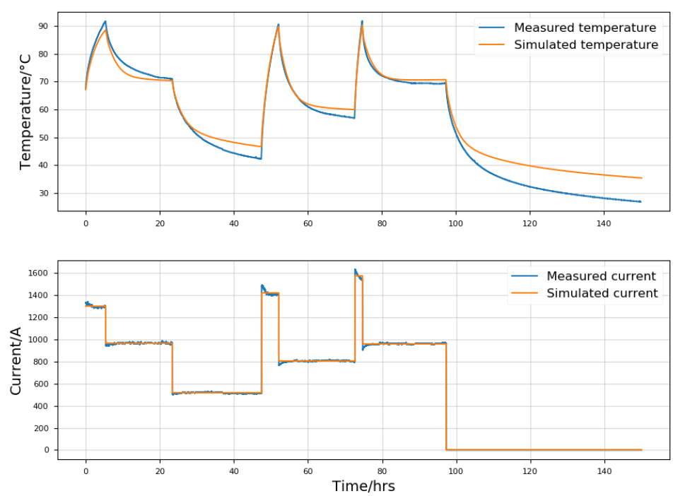
Figure 6 - Measured and calculated (IEC 60853-2 method) conductor temperatures
4.3. Comparison with purpose-built model
The model attempted to predict the entire sequence, starting from ambient temperature. The results are shown in Figure 7.
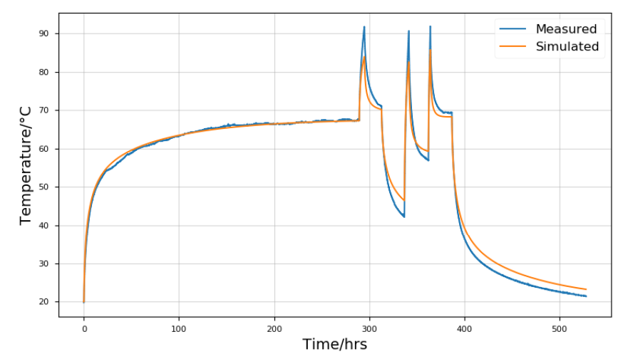
Figure 7 - Results from simulating with purpose-built model
The difference between the measured data and the predictions of the model at the peaks is approximately 6 °C.
4.4. Comparison with Finite Element model
In this section the measured conductor temperature is compared with a numerical model, where G(t) (see section 3) is calculated with the Finite Element software package Flux. This enables fast and accurate numerical calculations of the temperature at any position in the system for an arbitrary load pattern.
The finite element model is only used to determine the functions Gkl(t), whilst the cable losses are calculated with the same method as in section 4.2. It is assumed that the armour properties are constant with current. This approach will underestimate the losses for high currents, possibly explaining the small differences in the peak temperatures, especially after the period with maximum current (1574 A).
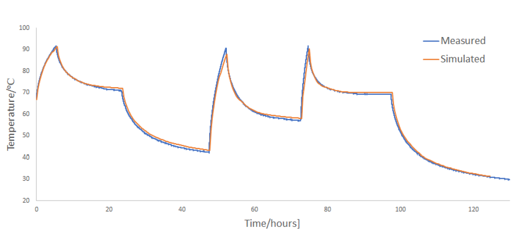
Figure 8 - Results from simulating with the Finite Element method
5. Discussion
The collected data show that the environment around the cable responds as expected to long-term load variations (days, weeks). For example, the temperature 45 cm from the cable surface idles about 5 °C above ambient. However, there is virtually no response to short-term loads (hours) at the same location. As a result, one could approximate the response to short-term loads while only considering the immediate surroundings. Note that this result is currently limited to the specific case at hand, and that more work is needed for it to be generalizable.
The IEC extrapolation method deviated from the first peak by approximately 3 °C, but it showed a noticeable improvement on the two latter peaks. The root cause of this inconsistency is unclear, but a probable cause is the cooling. The method’s cooling lagged behind the measured temperature, which resulted in a higher initial temperature on the last two high-load steps. In other words: Had the initial temperature matched with the real data before the two final high-load transients, the IEC method would have deviated from the peak.
That raises the question of why the cooling periods are lagging behind the measured data. It was found that the IEC method has an inconsistency for AC cables, with nonzero losses in screen and armour. When the loss factors are updated as a function of temperature, this inconsistency may lead to large errors, especially in the cooling periods, which may accumulate in subsequent periods of heating.
An option would be to use constant loss factors, however, since the screen and armour losses may change quite significantly with temperature this will not give a very accurate solution. A conservative estimate of the conductor temperature is obtained if the loss factors at low temperature are used for the entire dynamic rating.
The purpose-built model did not perform as well as the IEC method (deviating by approximately 6 °C at the peaks). It predicted the initial steady-state temperature well, while undershooting the short-term transients noticeably during the heating periods. An offset between measured and predicted initial temperature will impact the shape and—if it is a short-term transient—the endpoint of the transient. This error will accumulate with each short-term step, but it might vanish (be “reset”) if the system reaches an equilibrium temperature. The correct prediction of the initial steady state supports this hypothesis.
The initial error has yet to be explained (first peak). If the values for thermal capacity are too high, that would certainly contribute to dampening short-term transients. This model also keeps track of the entire thermal profile of the cable; if the predicted thermal profile (distribution of temperature) is incorrect, it would change the thermal response. For example, if the insulation layer is too cold initially, the heat would dissipate from the conductor faster (since heat flux is driven by difference in temperature).
To summarize: A general recommendation, based on these observations, is to gain more insight into the thermal properties of the materials used in XLPE submarine cables. Seemingly insignificant changes in the input parameters can cause significant changes in the output when predicting short-term, rapidly-changing transients. The results presented in this article do however intimate that load cycles can be modelled with relatively simple methods. This, along with the relevant input parameters, will need to be investigated further. Well-established (albeit more complicated methods) such as finite element modelling showed promising results.
References
- IEC 60853-2 Calculation of the cyclic and emergency current rating of cables. Part 2: Cyclic rating of cables greater than 18/30 (36) kV and emergency ratings for cables of all voltages
- P. Maioli, M. Bechis, G. Dell’Anna – AC Resistance of Submarine Cables – Jicable ’15 E5.2
- M. M. Hatlo et al. – Accurate analytical formula for calculation of losses in three-core submarine cables – Jicable ’15 E2.5
- R. Stølan, M. M. Hatlo – Armour Loss in Three Core Submarine Cables-Measurements of Cable Impedance and Armour Wire Permeability – CIGRE 2018, B1-306
Appendix - Thermocouple details
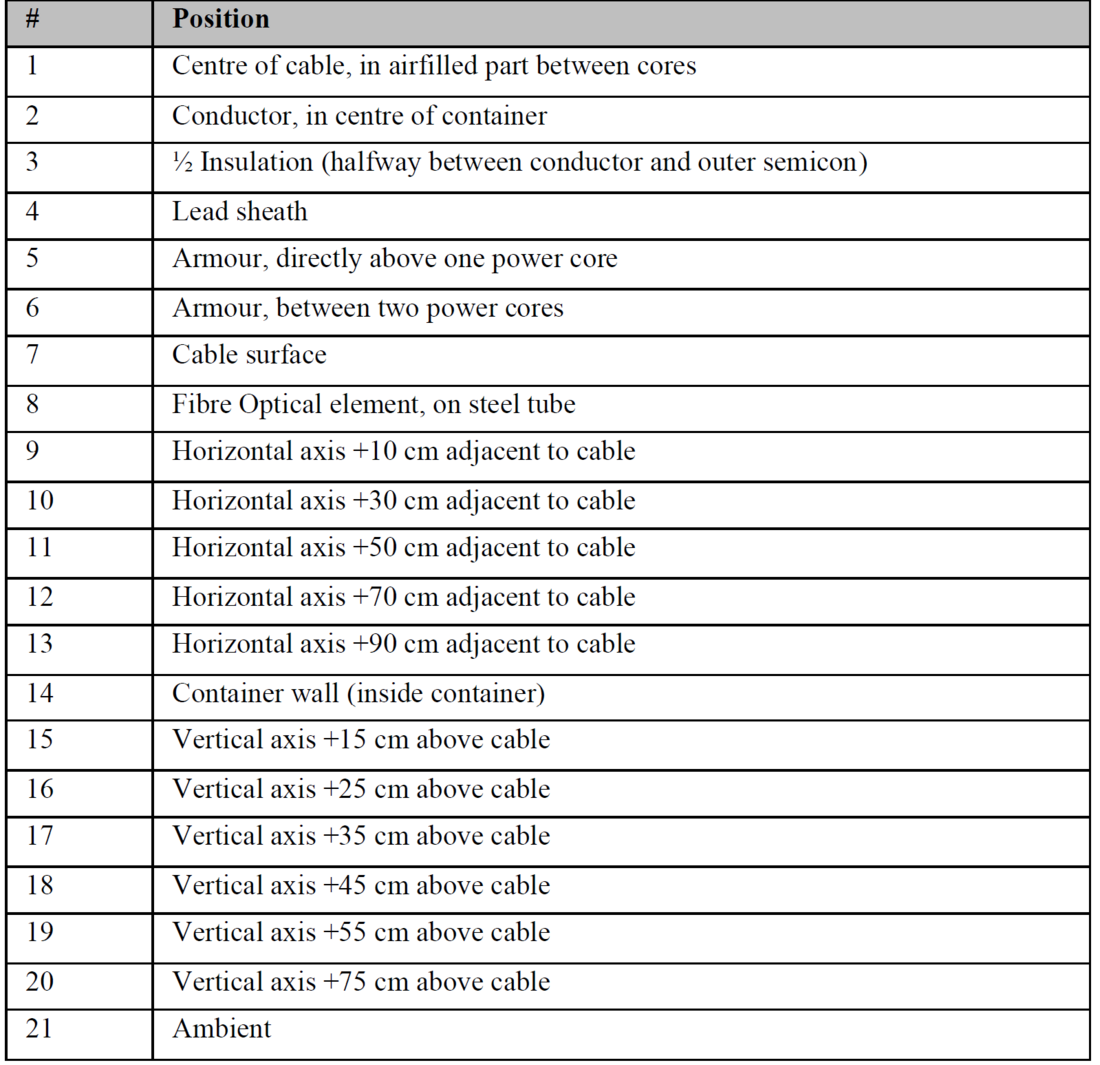
Table 3 - Overview of thermocouples
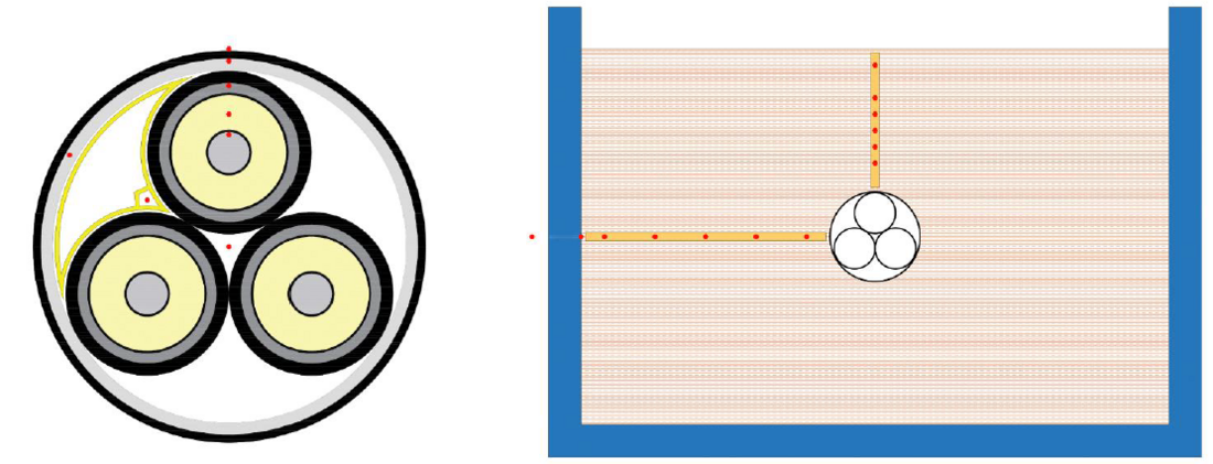
Figure 9 - Thermocouples positions in relation to the power cable and the test tank