A2 - Impact of Transient Voltage Generated by Valve Commutation on HVDC Transformer
Authors
Dr. R. WIMMER, T. HAMMER, T. MANTHE, V. HUSSENNETHER, Marcus HÄUSLER - Siemens Energy, Germany
Z. CHI, W. RUAN - Siemens Energy, China
T. STROF, S. REHKOPF, M. BENGLER, A. PALANI - Maschinenfabrik Reinhausen, Germany

Summary
The purpose of the investigation presented in this paper was to find out transient coupling effects between converter and tap winding due to the commutation process of the valves. It is known that the commutation process of the valves leads to voltage drops in the voltage between the transformer and the valves. These voltage drops are perceived by the transformer as a repetitive, transient signal. Due to the inductive and capacitive couplings between valve- and line- / tap-winding, the transient signal couples to the tap winding and creates additional dielectric stress. In past this phenomenon is well covered by the insolation coordination. However, the power and voltages of HVDC transformers increase and the question comes up if this phenomenon is still covered by conventional insulation coordination. Taking the example of a 400 kV DC / 1050 kV AC / 493 MVA HVDC transformer these phenomena are investigated in more detail.
The investigation is split into three parts:
- Simulation of a converter with a simplified transformer model to get out corresponding voltage / current shapes at 3 different operation modes:
- Operation mode 1: nominal load with extinction angle gamma in nominal range
- Operation mode 2: partial load with extinction angle gamma in nominal range
- Operation mode 3: short time operation at 70° firing angle.
To reduce the complexity of the simulation model only a typical six-pulse group is used.
- Detailed simulation of transformer to check the transient coupling between valve winding and tap winding. Here, the 3 simulated voltage / current shapes of the six-pulse group converter are taken as extinction signal. To get meaningful simulation results also the transformer-terminals were integrated into simulation model.
- Verification of the transformer simulation model. Here, the transformer was excited with a transient signal which steepness corresponds to the transient signals which were simulated in the converter model. Care was taken to ensure that the same connection configuration is used as with the transformer simulation in point 2. At this measurement it was possible to measure directly the voltage of one step of the line side tap winding.
The results of the measurements confirm the applicability of the simulation model to study transient effects within transformer caused e.g., by the commutation process of the valves. The simulation of such transient effects confirms also appropriate dielectric strength inside of the transformer. Finally, it was found out that all dielectric stresses are covered by the common approach to determine the insulation coordination for this transformer. No modification or additional dielectric aspects needs to be considered for a safe, reliable and continuous operation of the transformer.
Keywords
HVDC transformer - transient signal - commutation process - coupling effects - simulation model - transient measurements1. Introduction
One classical field of High Voltage Direct Current transmission (HVDC transmission) is the bulk power transmission over long distances. Currently power ratings of 12 GW at 1100 kV and 10 GW at 800 kV are possible and were already realized. Now, for the first time in 2018, a regulated HVDC transformer was directly connected to the UHV AC system (Ultra High Voltage AC System).
The transformer valve side voltage does not show an ideal sinus wave. Due to the commutation process of the valves the voltage shows several voltage-drops within one sinus period. These voltage drops can be seen as transient distortions. Consequently, the transformer is constantly exposed to these transient signals. By complying with relevant standards (e.g. IEC 60071-5 [IEC 60071-5] for thyristor valves, IEC 60099-9 [IEC 60099-9] for surge arrester (HVDC), IEC 61378 resp. IEC 60076-57-129 [IEC 61378 & IEC 60076-57-129] for HVDC transformer) and choosing suitable insulation coordination, this problem is successfully countered. Additionally, the interaction of valve commutation and the voltage profile for HVDC transformer which has a typical transmission voltage up to 600 kV DC and up to 550 kV AC on the line side is well described in the CIGRE brochure [CIGRE-Br. - 2015].
However, the line-side voltage of previous HVDC transformers is typically in the range between 420 kV and 525 kV. Now, the line side voltage is doubled to 1050 kV, while the step voltage for the regulations is kept at nearly 4 kV. All windings of the 1050-kV-AC-HVDC transformer are designed according to the insulation coordination rules by the transformer manufacturer and have been checked regarding the resulting transient requirements, too. However, for such kind of transformer there is only limited experience available regarding transient coupling effects from the valve winding to the tap winding. To ensure a safe and reliable operation of the transformer the impact on the tap winding or OLTC due to the transient signal generated by the commutation process needs to be investigated in more detail.
2. Simulations of converter
Task of the present work is to observe the transients caused by the valve commutation process for steady state operation at the tap winding. For the simulations, the following 2-step approach as outlined in chapter 2 and chapter 3 is used:
Chapter 2 summarizes calculation of valve side voltages profile derived with a detailed valve representation and a simplistic model of the converter transformer which includes the main inductance and the stray capacitances as a lumped circuit. This approach is in line with the transformer model in the CIGRE brochure [CIGRE-Br. - 2015]. Thus, chapter 2 serves to derive the correct voltage profile at the converter transformer valve side terminals.
In chapter 3 the valve side voltages calculated in chapter 2 are used as a voltage source applied to a detailed model of the converter transformer. Using the detailed converter transformer representation allows a closer look at the voltage distribution within the converter transformer and especially at the stresses acting on the lines-side tap winding and connected OLTC (on-load tap changer).
2.1. Converter Model
The investigations are performed on a Line Commutated Converter (LCC) bipolar system for which each pole is made up of two series-connected 12 pulse valve groups. For the studied project the upper “800 kV DC” valve group and the lower “400 kV DC” valve group are connected to two different AC systems. Each 12-pulse group consists of the well-known serial connection of two 6-pulse groups which are connected via YY and YD converter transformers to the AC systems. The focus of this study is on YY converter transformers of the 400 kV DC valve group being connected to an HVAC system with system voltage of 1050 kV AC. The basic operating principle of LCC converters and especially the interaction of the valves with the converter transformers during the commutation process are well described in [Arrilaga - 1998]. The OLTC positioned on the HV network side of the converter transformers plays a vital role for operation of LCC schemes since it is operated to control firing angle within predefined operating limits for the individual operating points.
Figure 2-1 shows the equivalent circuit of one 6-pulse group used for modelling the commutation process. Table 2-1 explains the abbreviation acc. to Figure 2-1. Such a model represents accurately the commutation process within one 6-pulse group and thus allows to represent the highest transient voltages of the specific commutation process. Further extension of the model to represent the entire bipolar scheme as combination of multiple 6-pulse models is straightforward and may be used for further refinement including cross coupling effects of the adjacent 6-pulse bridges. Double valves represent a Multiple Valve Unit (MVU). Six Multiple Valve Units are used to form one 12 pulse bridge. The valves are constructed from repeated valve sections which have the same electrical characteristics as the complete valve, but only a fraction of the voltage-withstand capability. Each valve section consists of thyristor levels and valve reactors connected in series.
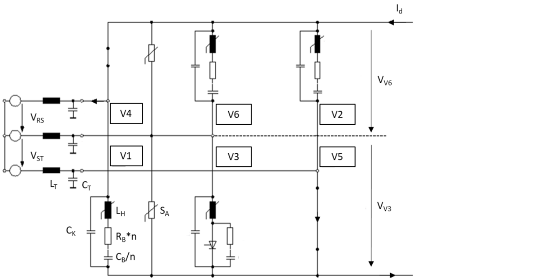
Figure 2-1 - Basic representation of the complete simulation model
| VRS, VST, VTR | Phase-to-Phase Voltages Line Side |
| LT | Converter Transformer Impedance |
| V1 … V6 | Converter Valves |
| SA | Surge Arrester |
| LH | Saturable Valve Reactor |
| n | Number of Thyristor Levels |
| RB | Snubber Resistor |
| CB | Snubber Capacitor |
| CK | Grading Capacitor |
| VV1 ... VV6 | Valve Voltages |
| Id | DC Line Current |
The non-linear reactor reduces the di/dt turn-on stress at valve firing as well as the voltage stress on the thyristor levels at steep fronted surges, both during disturbances and normal commutation. This function is assisted by the RC snubber circuits associated with each thyristor level. Another function of the RC snubber circuit is to limit the commutation overshoot voltage stressing the thyristor during turn-off operation of the valve and to linearize the voltage distribution between thyristors for power frequency and switching-surge-type voltage stresses. An arrester is installed in parallel to the valve, which limits external overvoltage’s and excessive commutation overshoot voltages for high firing angles.
2.2. Selected Operating Points and Results of the Simulation
Table 2-2 summarizes the valve properties and Table 2-3 the three representative operating points selected for this study. For nominal and partial load typical rectifier operating points for steady state operation are selected. The third operating point is a quasi-stationary operating point needed when bringing a second 12-pulse group into service. The valve operating point for this scenario requires a limited DC voltage generation of a 12-pulse group which is realized via high firing angles. It is selected to represent intermediate quasi-stationary operation of the valves which may persists at least for couple of minutes to allow for coordination between the sending and receiving station.
The results of simulations performed using the model shown in Figure 2-1 are the phase-to-phase valve side voltages at the converter transformer valve side terminals which are used as input for further simulations discussed in chapter 3. The valve side phase-to-phase voltages are shown summarized in Figure 2-2 for the three operating points defined in Table 2-3. There it is visible that the deblock of the 2nd group shows the highest transient voltages. Here dU/dt is at 37 kV/μs which correspondence to a wave-front duration of T1 ≈ 6.8 μs at a maximum peak voltage of 250 kV.
| LCC Valves | |
| No. of Series Connected Thyristor Levels | 60 |
| No. of Valve Reactors | 8 |
| Snubber Circuit | CB = 1.6 μF/n RB= 36 Ω*n |
| LCC Operating Points | DC Line Current Id | Firing Angle of Valves α |
|---|---|---|
| Nominal Load: | 6250 ADC | 15° |
| Partial Load: | 2800 ADC | 18° |
| Deblock 2nd Group: | 6250 ADC | 70° |
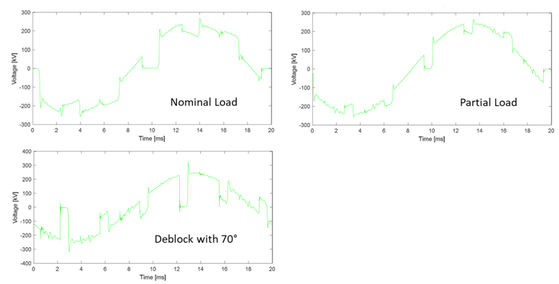
Figure 2-2 - Results of the commutation simulation
3. Transient simulation of transformer
The most important questions with the results from chapter 2 were to study the impact of such voltages with transient voltage drops on the insulation coordination inside the transformer and additionally if there is an unexpected high transferred voltage from converter- to line-side inside the transformer. Therefore, a high frequency model of a HVDC transformer was created. On this transformer model were applied the converter voltages for all three operation modes.
3.1. General Data of Transformer
Table 3-1 summarizes the general data and main parameter of the chosen HVDC transformer.
| Rated Capacity: | 493.1 MVA |
| Cooling Type: | ODAF |
| Frequency: | 50 Hz |
| Phase: | single phase |
| Rated Voltage of Line Winding: | 1050/√3=606.2(+21 -9 steps*0.65% kV each) |
| Rated Voltage of Valve Winding: | 167.4/√3=96.42 kV |
| Rated current of Line Winding: | 813 A |
| Rated current of Valve Winding: | 5102 A |
| Impedance at Nominal Tap: | 20% |
| Position of Test Terminal: | 1.9 |
| Test Location: | Test bay of transformer manufacturer |
3.2. Model Description
The high frequency model of the transformer is based on white-box approach mentioned in the Cigré brochure [Cigré-Br. - 2014]. Such a white-box model is a detailed model, developed from physical geometry of transformer windings and material characteristics. The used type of white-box model is the lumped parameter model, that is built from circuit parameters as self- and mutual inductances, capacitances and resistances. The software to generate this lumped parameter model is a manufacturer inhouse tool, typically used at the development stage.
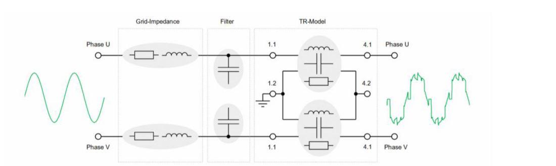
Figure 3-1 - Basic representation of the complete simulation model
The applied transformer model is valid for a frequency up to 1 MHz. It considers only a single limb of the 1-phase-transformer. The model includes all windings and is created for a defined tap-position. The transformer model was extended by some elements like the AC-filter and a grid impedance. The star point of the converter side is open and on the 1050-kV-side grounded. A sinusoidal phase-to-phase voltage is applied at the terminals of the AC-grid side and the simulated phase-to-phase voltage for the three different operation modes is applied at the terminals of the converter side. An overview of the complex model is shown in Figure 3-1.
This complex model has a few restrictions, e.g. grounded loops and connections between transformer, filter and grid impedance are not modeled.
3.3. Simulation Results
This chapter summaries some simulation results for all three operation modes. All presented results are focused on the transferred voltage on the tap winding. The Figure 3-2 to Figure 3-4 shows the time characteristic of the voltage drop across one step (tap 1.8 – 1.9) of the tap winding.
Figure 3-2: This figure shows the results for operation mode 1: nominal load with extinction angle gamma in nominal range.
Figure 3-3: This figure shows the results for operation mode 2: partial load with extinction angle gamma in nominal range
Figure 3-3: This figure shows the result for operation mode 3: deblock with 70° firing angle.
Transient oscillations with a minor peak value and a resonance frequency of about 50 kHz could be observed at all three operation modes. This resonance frequency is in the typical range of the natural frequency of tap windings.
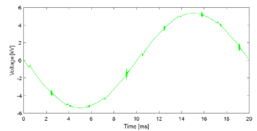
Figure 3-2 - Time characteristic of the voltage drop across one step of the tap winding for mode1
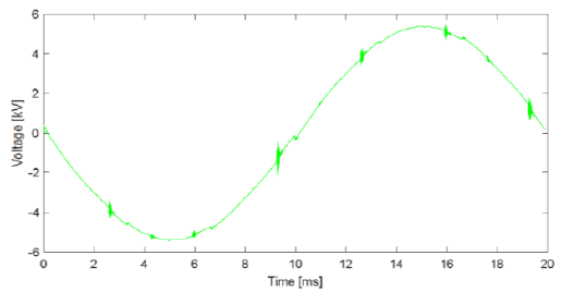
Figure 3-3 - Time characteristic of the voltage drop across one step of the tap winding for mode2
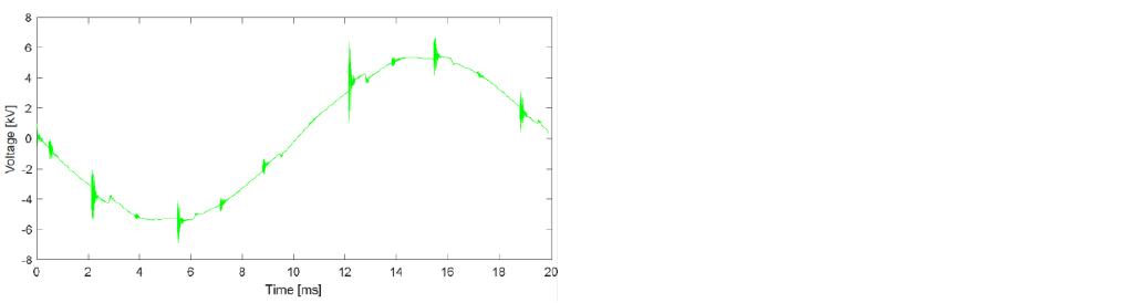
Figure 3-4 - Time characteristic of the voltage drop across one step of the tap winding for mode3
3.4. Conclusion
The simulation with a high frequency model of a HVDV transformer for the three operation modes of the HVDC converter station shows the following results:
With respect to the commutation at the converter station, transient voltages across one step of the tap winding can be observed in general. For practical continuously operation cases of the HVDC converter station (operation mode 1 and 2) a relevant effect of these transient voltages to the step voltage of the tap winding could not be detected. For practical short time operation cases of the HVDC converter station (operation mode 3) a temporary increase of the step voltage of the tap winding through transient voltages in the range up to 1.2 p.u. could be simulated. The step voltage increase is quite low compared to the load applied during the successfully passed factory acceptance test. The induced voltage test (IVPD) according to [ICE 60076-3] has AC-voltage of 1.82 p.u. for 5min and 1.58 p.u. for 60 min.
4. Transient measurements on transformer
The purpose of this investigation was to verify the simulation model of the transformer. Therefore, the transformer was excited on the valve side with a defined impulse voltage and the response signal was measured between defined taps of the tap winding on the line side. Afterwards the measurement results were compared with the results of the simulation.
4.1. Condition of Transformer
The special transient voltage measurements were carried out after the FAT of the transformer was successful finished. The diverter switch was modified to measure the transient voltage signal directly between the diverter switch contacts in their final open position, details see chapter 4.2. After these measurements the modifications were removed. To ensure highest quality of the product some dielectric tests of FAT were repeated. One of these tests is the IVPD. The criterion for this test is that the PD show the same good behavior compared to the original FAT and not only to be lower than the required limit.
The transformer was tested with an AC voltage of 1100 kV for 5 min and 953 kV for 60 min including PD measurements. The voltage along the tap winding is:
72.2 kV + 43.3 kV = 115.5 kV for 5 min
and
62.6 kV + 37.5 kV = 100.1 kV for 60 min.
The tap winding consists of 17 taps which means 16 voltage steps. The resulting voltage between two next-to-next taps is:
115.5 ??16 = 7.2 ?????=> 7.2 ????? ∙ √2 ≈ 10.2 ?????? ??? 5 ???
100.1 ??16 = 6.3 ?????=> 6.3 ????? ∙ √2 ≈ 8.8 ?????? ??? 60 ???
The PD measurements did not show any abnormalities. So, the a0 distance of the diverter switch safely withstands 10.2 kVpeak for 5 min and 8.8 kVpeak for 60 min.
4.2. Test Circuit and Coupling Out of Transient Signals on the Tap Changer
Figure 4-1 shows the test circuit to couple out transient signals at the tap changer. It is visible that two possibilities are given:
- Without preparation of the diverter switch by using the tap lead 1.9 via auxiliary bushing (blue drawn circuit in Figure 4-1)
- With prepared diverter switch (red drawn circuit in Figure 4-1)
At the measurement with prepared diverter switch no signal was measured on tap connection 1.9. However, the capacitive voltage divider was still connected on tap connection 1.9. The test circuits are described in more detail in chapter 0 and chapter 4.2.2.
At this investigation the voltage drops on the converter side are of interest. According to the simulation results of chapter 2 and 3 the short time operation mode at 70° firing angle shows the highest stress for the windings. Consequently, the transformer needs to be excited with a similar transient signal like the voltage drops visible in Figure 2-2. For that reason, an impulse of max. 250 kV amplitude, a front time of T1 ≈ 6.8 μs and a tail time of T2 ≈ 225 μs are applied on the converter winding of the transformer.
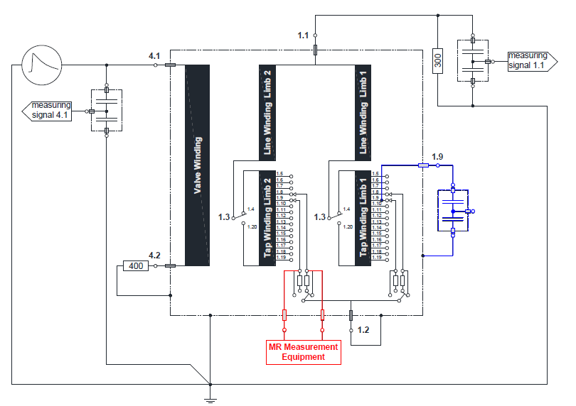
Figure 4-1 - Test circuit with (red drawn circuit) and without (blue drawn circuit) prepared diverter switch
4.2.1. Without prepared Diverter Switch
The tap connection 1.9 was led out for testing reason (see also Figure 4-1 blue drawn circuit). This exit lead can be used to measure the occurring voltage to earth. To measure the voltage of one step it is important that the tap position is on 10 or 12 (tap connection 1.10 or 1.8) and the neutral point line side is earthed. The tap position 12 (tap connection 1.8) was chosen for further investigations.
This exit lead is also still existing during operation. For that reason, it is designed for all kind of dielectric stresses which occurs during testing and so it fulfills all insulation requirements of the transformer. On the tank wall a drip-proof seal is assembled which ensures that an auxiliary bushing can be assembled / disassembled while the transformer is filled with oil. The auxiliary bushing is typically a normal DIN oil-bushing (without capacitive control) and is mounted on the longitudinal tank wall of the valve side. The signals on the terminal of this bushing will be transmitted with an unshielded wire (cross section: 2.5 mm², length: ~2 m) to a capacitive voltage divider. A coaxial cable (RG214) transmits the signal from the voltage divider to the transient recorder of the transformer manufacturers test bay. Here, the signals are recorded with a resolution of 12 bit, a sample rate of 200 MS/s and a time length of nearly 350μs.
Important note: To avoid any circulating current problem, it is forbidden to connect the wires of parallel connected windings before the tap changer. For that reason, only the tap lead 1.9 from limb one is guided out of the transformer.
4.2.2. With prepared Diverter Switch
The voltage between the diverter switch contacts in their final open position is defined here as distance a0. To measure directly at that distance a0 it is necessary to take out the diverter switch from the transformer and assemble adequate cabling and bushing on the diverter switch. After this preparation the diverter switch is installed again into the transformer. Two broadband high voltage divider and two A/D converter are placed on the top of the transformer. The test equipment is designed for 20 kV AC and a lightning impulse of up to 70 kV.
The A/D converter shows following performance: 14 bit resolution and a sample rate of 100 MS/s. The operation of the A/D converter is done with 230 V power supply and an isolating transformer. The digitized data are transmitted to the transient recorder which records the data after a trigger event. Afterwards the recorded data are transmitted to a personal computer or Laptop.
Important note: The measurement equipment is mounted on sector 3 of the tap changer. This sector is linked to the tap winding on limb 2.
4.3. Analysis of Measured Signal and Comparison to Simulated Signal
This chapter discusses the comparison between measured and simulated results of the transferred impulse to tap winding. The used simulation model for the transformer was described in the chapter 3. This model was adjusted by the used test components, e.g. the leads and the voltage diverter.
4.3.1. Analysis of Measured Signal at Terminal 1.9
Figure 4-2 shows the measured signal of the applied voltage on the terminal 4.1 (impulse on valve winding), the measured signal of the transferred voltage on the tap winding terminal 1.9 and therefore over one step of the tap winding and the measured signal of the transferred voltage on the line winding terminal 1.1. The analysis of the response signal on terminal 1.1 and 1.9 shows:
Up to 10 μs:
In the first 10 μs a very fast transient peak and high-frequency oscillations can be recognized for both response signals. This area is zoomed out in Figure 4-3. Here, the voltage at terminal 1.9 shows two dominant oscillations: One oscillation in the time range of -0.5 μs up to 2.5 μs which has a frequency of ~1.2 MHz and one in the time range of -0.5 μs up to 0.3 μs which a has frequency of ~10 MHz. The maximum voltage amplitudes are: +2230 V and -3710 V. Similar observations can be made for the measured voltage on terminal 1.1. This signal also shows two dominant frequencies: One oscillation at ~1.3 MHz in the time range -0.5 μs up to 8 μs and one oscillation at ~11 MHz in the time range of -0.5 μs up to 0.7 μs. The maximum voltage amplitude is: -22.1 kV.
These high frequencies of both signals are not explainable with the applied impulse, because the front time of the applied impulse is only 6.8 μs. Such a front time suggests an analyzable frequency of approx. 1/Tfront = 1/6.8 μs ≈ 150 kHz. In fact, the spectrum analysis shows that the SNR (Signal-to-Noise Ratio) for such front times becomes too low for frequencies higher than 200 kHz. Consequently, the observed high frequency oscillations at the beginning are caused by the outer measurement circuit e.g. reflections in the measurement circuit and potential equalization in the earthing circuit. The influence of the measurement circuit on measured signals are well described in “Reproducibility of Transfer Function Results” and “The influence of connection and grounding technique on the repeatability of FRA-results” [Wimmer-2003, Wimmer-2007]. For that reason, the first 10 μs are only of limited value for evaluation.
From 10 μs until end of record length:
The analysis of the transferred voltage on the tap winding terminal 1.9 show a strong distinct oscillation of the tap winding at ~16.3 kHz. Two essential frequencies at ~7.74 kHz and ~40 kHz are superposed at this basis oscillation. Further essential natural frequencies at ~35.2 kHz and ~50 kHz are also modulated on this dominant natural frequencies of the tap winding. No other essential natural frequencies could be detected up to 200 kHz. The maximum voltage amplitudes are reduced to +660 V and -1220 V. The transferred voltage on the line winding terminal 1.1 shows a dominant natural frequency at ~8.6 kHz and further light distinct frequencies, which are lower than 50 kHz. The maximum voltage amplitude is reduced to -20.7 kV.
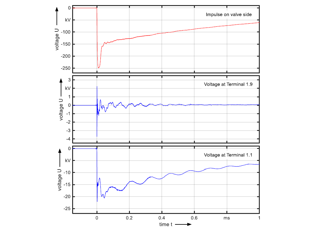
Figure 4-2 - Measured voltage-signals
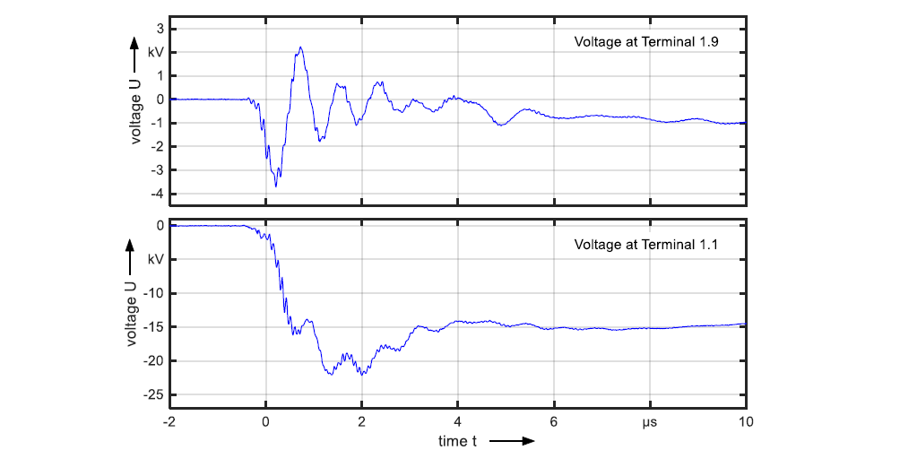
Figure 4-3 - Zoomed area of voltages on terminal 1.1 and 1.9
The signals at terminal 1.9 and terminal 1.1 are not similar to each other. That means between terminal 1.1 and terminal 1.9 (which corresponds to the voltage at the distance a0 of the tap changer) exists a complex electric network. Consequently, it is not possible to draw easily conclusion about the signal occurring at the distance a0 of the tap changer by measuring the signal at terminal 1.1.
4.3.2. Transferred Impulse Signal Measured at Terminal 1.9 vs. Directly Measured at a0
As already mentioned at the beginning of chapter 4.2, the response signal along one step of the tap winding is measured using different methods. In both cases tap position 12 was selected to enable a comparison of these two measured signals. Figure 4-4 shows the comparison between measured signal of the transferred impulse to tap winding at terminal 1.9 and the direct measured transferred impulse at distance a0.
Up to 10 μs:
Figure 4-5 shows the comparison of both response signals up to 10 μs. The signal sequence deviates significantly from the signal sequence measured on terminal 1.9, but it also shows frequencies higher than 1 MHz. As explained in chapter 4.3.1 this is only explainable by reflection and equalization processes of the outer measurement circuit. Consequently, the signal measured directly at distance a0 is exposed to the same effects as the signal measured at terminal 1.9.
The maximum voltage amplitude for the signals directly measured at distance a0 are: -1530 V and +1180 V and are lower than the maximum voltage of the signals measured on terminal 1.9 (-3710 V and +2230 V).
The different signal sequences are logic and can be explained with the different test circuit, which leads to a different reflection and equalization processes. Consequently, the natural frequencies are different as well as the amplitude of the signal curve.
From 10 μs until end of record length:
Here, it is visible that the signals are similar to each other. The corresponding natural frequencies of the signal directly measured at distance a0 are: ~7.88 kHz, ~16.3 kHz, ~34.8 kHz, ~40 kHz and ~50 kHz.
Also here, no other essential natural frequencies could be detected up to 200 kHz. These natural frequencies correspond well to the natural frequencies of the response signal which are measured at terminal 1.9 (see Table 4-1). The maximum voltage amplitudes are reduced to -1220 V and +880 V.
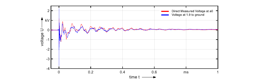
Figure 4-4 - Comparison of the two different measured response signal up to 1 ms
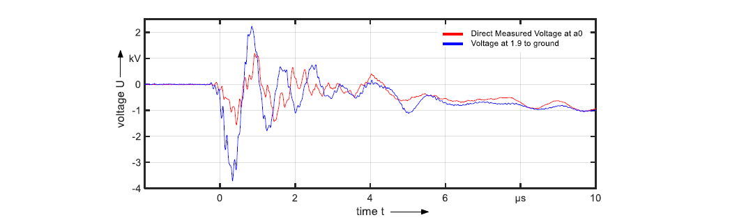
Figure 4-5 - Comparison of the two different measured response signal in the first 10 μs
The obvious differences of the signals are explainable with the following facts:
- The measurements of both approaches are not carried out at the same limb. This has the consequence that the length and the position of the exits leads of the tap winding are different which results in another RLC-network.
- The measurement circuit of both approaches are also different. The directly measured signal uses unshielded wire from the connection of the distance a0 to the broadband high voltage divider outside the transformer. The broadband high voltage dividers imply an additional capacitive loading for the system. Consequently, the RLC network of the transformer system is influenced by the measurement setup.
- The measurement equipment for the direct measurement at distance a0 was not applied during the measurement using the terminal 1.9.
Due to these facts, it could not be expected that the signal curves of both measurement approaches are congruent. Nevertheless, the curves show a very good accordance regarding the oscillation behavior. As already mentioned in chapter 4.3.1 an evaluation higher than 200 kHz doesn’t make sense because the SNR of the exciting signal becomes low for frequencies higher than 200kHz. Frequencies which can be recognized at higher frequencies are generated by reflection or potential equalization.
| Natural Frequency in kHz | |||||
|---|---|---|---|---|---|
| Direct Measured Signal | 7.88 | 16.3 | 34.8 | 40 | 50 |
| Measurement at Terminal 1.9 | 7.74 | 16.3 | 35.2 | 40 | 50 |
The voltage amplitude of the direct measured signal for records >10 μs have a maximum amplitude -1220 V and +880 V. Table 4-2 compares the voltage amplitude of the direct measured response signal and the response signal measured at terminal 1.9 for records >10 μs. Here, also the voltage amplitude shows a good accordance. While the negative voltage amplitude has the same value the positive voltage amplitude shows a slight deviation. However, the amplitudes of the response signal are low compared to the amplitude of the input signal, which is 250 kV. The response signals have a maximum amplitude of only 0.49% of the applied impulse.
| Max. Voltage without the first 10μs | Ratio of max. Voltage without the first 10μs to applied Impulse (250 kV) | |||
| Negative Range | Positive Range | Negative Range | Positive Range | |
| Direct Measured Signal | - 1.22 kV | +0.88 kV | 0.49% | 0.35% |
| Measurement at Terminal 1.9 | - 1.22 kV | +0.66 kV | 0.49% | 0.26% |
4.3.3. Comparison to Simulated Signal
The target in chapter 3 was to clarify transient commutations effects on the converter side of the transformer on the tap winding for a normal operation case. Such investigations cannot be performed on site easily. For that reason, the effects are carried out with a simulation model. The most important goal here was to evaluate the maximum voltage stress which occurs between taps. As already described the measuring circuit influences the measuring results. Consequently, the simulation model of the transformer needs to be extended with the RLC network of the measuring circuit. For that reason, important parameters like cable length, cross section, capacitance per unit length, capacitance of the voltage divider, etc. were recorded and the adequate values for measuring network were determined. Here the electrical network of the measuring circuit is replicated with simple, concentrated elements which are not further discretized which means the network of the measuring circuit did not show a high frequency resolution. In addition, frequency effects (e.g. skin effect) of earthing bands and leads are not considered.
The measured input signal was used as the input signal for the simulation. This ensures the comparability of the results between measured and simulated response signal.
Figure 4-6 shows the comparison of the measured and simulated voltage on the tap winding measured at terminal 1.9 to ground. It is visible that the simulation shows some deviations in the frequency behavior. The main natural frequencies of the simulation can be recognized at ~8 kHz, ~15 kHz, ~37 kHz, ~61 kHz. The comparison of the measured natural frequencies with simulated ones shows that the visible frequency deviation of the signal curves is just a shift. The simulated natural frequencies of the lower frequencies can be assigned very good to the measured frequencies (green cells of Table 4-3). For frequencies higher than 40 kHz an assignment of the natural frequencies is also possible (yellow-green cells of Table 4-3) but the shift is larger. Only the natural frequency at 35.2 kHz cannot be assigned (blue cell of Table 4-3).
The maximum voltages of the simulation are -2330 V and +2010 V. As already mentioned, the first 10 μs of the measured signal cannot be taken for signal analysis within the transformer. For that reason, the comparison of the max. voltage disregarded the spikes in the first 10 μs of the measured signal. The simulation did not show the typical high frequency oscillation in the first 10 μs due to reflection at ~1.2 MHz and ~10 MHz. Table 4-4 shows the summary of the comparison and reflect it to the maximum voltage peak from the input signal (ratio).
Explanation for natural frequency deviation:
The simulation model includes several simplifications:
- All external or internal leads are simulated with one concentrated element
- External used resistors, capacitive dividers are also simulated with one concentrated element
- The length of the leads and the distances to earth potential are only approximated. Installation tolerances are not considered. To determine the values the full cross-sections of the leads are considered. High frequency effects like the skin effect were not considered.
- Capacitance of bushing is also considered only as one concentrated element.
- The earth capacitance from the tap winding (outermost winding) to tank wall (earth potential) is estimated and simulated as rotationally symmetric which is in reality not the case.
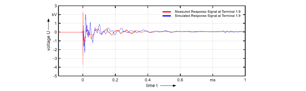
Figure 4-6 - Comparison of measured and simulated response signal at terminal 1.9
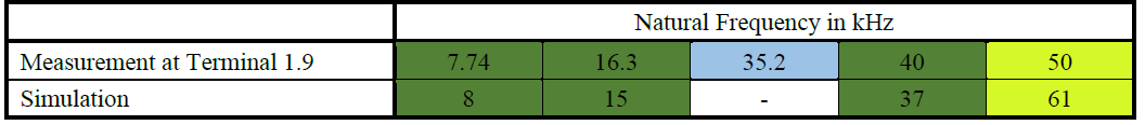
Table 4-3 - Summary of eigenfrequencies of the different approaches
| Max. Voltage without the first 10μs | Ratio of max. Voltage without the first 10μs to applied Impulse (250 kV) | |||
| Negative Range | Positive Range | Negative Range | Positive Range | |
| Measurement at Terminal 1.9 | - 1.22 kV | +0.66 kV | 0.49% | 0.26% |
| Simulation acc. "Meas. T 1.9" | - 2.33 kV | +2.01 kV | 0.93% | 0.8% |
4.4. Measurement Conclusion
Two different measurement concepts are used. The measurement at the test bushing (“Measurement at terminal 1.9”) is done by measuring one connection point (connection 1.9) to earth while the direct measured signal approach is done by measuring the voltage to ground on both ending points of the distance a0. Afterwards the difference between these two signals is formed mathematically and the voltage along the distance a0 is obtained. In addition, the “direct measured signal” approach did not show such strong reflection behavior than the “measurement at terminal 1.9” approach. However, the following facts can be summarized:
- Both measurements show the same maximum peak voltage in the relevant area.
- Both measurements show the same frequency behavior.
Consequently, the maximum measured peak as well as the frequency behavior can be trusted, independently which measurement approach is used.
The comparison of the measured natural frequencies with simulated one show a good accordance. All natural frequencies except the natural frequency at ~35.2 kHz can be assigned and show only small frequency shifts. This is remarkable in consideration of the simplifications of the simulation model. Consequently, the results calculated by the utilized simulation model can be trusted.
Since the reflections of the measuring system are not simulated the first 10 μs of the measured signal can be neglected for the comparison of the maximum voltage peak between measured and simulated signal. According to this, the simulated maximum voltage peaks are always higher than the measured value. In a direct comparison, the simulated values are higher in the range from 50 % to 95 % than the measured values. This seems high, but it must be considered that the amplitude of the response signal is just 0.26 % up to 0.93 % of the exciting level. That means the simulation model needs to provide in per mill area exact values, which is not so easy to implement.
Since it is primarily a question of voltages stress and not of frequency accuracy, the voltage amplitude is of higher importance. The comparison of measurement and simulation shows satisfactory match of the results. More importantly, the simulation model shows higher amplitude values. Consequently, the simulated, transferred, transient signals from the valve side to the tap winding can be considered as a worst case.
5. Further investigations
In addition to the investigation of transferred transient signals the voltage characteristic at the distance a0 at the diverter switch was also recorded during the switching event of the tap changer at load and no-load losses test of the transformer. No inadmissibly high transient voltage peaks could be observed here. In general, the basic curve is very similar to the voltage curves presented in " On-site Transient Recovery Voltage (TRV) Measurement in OLTC with Vacuum Interrupter in Comparison with Simulation Results" [Gebauer - 2013].
6. Conclusion
The investigations carried out in this paper support that the insulation coordination rules utilized by the transformer manufacturer are sufficient to ensure an appropriate high dielectric safety margin within the transformer for a safe, reliable and uninterrupted operation of the transformer, even with HVDC/UHVAC transformers. Consequently, it is not necessary to take care of further aspects concerning the insulation coordination for projects which are equal to the project presented in this paper.
In this investigation no additional parameter could be identified which needs to be considered in addition in the simulation model. The commutation overshoot depends on the stray capacitance, inductance and other parameter described in the CIGRE brochure [CIGRE Br. - 2015]. These parameters change at different projects. For that reason, the results cannot be transferred one-by-one to other projects.
The simulations have shown that the commutation overshoot of the valves have no significant effect on transient voltages on the tap winding at the 1050-kV-line-side of the transformer. The voltage drops on individual steps of the tap winding fit very well the sinusoidal shape. Just small transient voltages in a range of about 300 V superimposed to the 50-Hz-voltage can be observed. These superimposed voltage peaks are in a voltage range that leads to a high safety margin in comparison to permissible voltage.
The comparison of the measured transient signal and the transient signal out of the transformer simulation show some differences in amplitude and frequencies.
Reasons for those differences are some simplifications in the simulation model and that not all parasitic effects are considered. However, the amplitudes out of the simulated signals always shows a higher value than the amplitude of the measured signals. Therefore, the simulation model in this paper can be regarded as a conservative approach. In fact, the voltage values from the coupling effects will be lower than the simulated ones.
References
- IEC 60071-5 Insulation co-ordination - Part 5: Procedures for high-voltage direct current (HVDC) converter stations
- IEC 60099-9 Surge arresters - Part 9: Metal-oxide surge arresters without gaps for HVDC converter stations
- IEC 61378 Converter transformers - Part 1: Transformers for industrial applications / Part 2: Transformers for HVDC applications / Part 3: Application guide
- IEC 60076-57-129 Power transformers - Part 57-129: Transformers for HVDC applications
- CIGRE Technical Brochure 577, “Electrical Transient Interaction between Transformer and the Power System: part 1 - Expertise”, Joint Working Group A2/C4 39, April 2014
- CIGRE Technical Brochure 609, “Study of Converter Transients Imposed on the HVDC Converter Transformer”, Working Group B4.51, February 2015
- J. Arrillaga, High Voltage Direct Current Transmission, Institution of Engineering and Technology, 1998.
- R. Wimmer, K. Feser, J. Christian “Reproducibility of Transfer Function Results” - 13th Int. Symp. on High Voltage Engineering (ISH), 2003, Paper 165
- R. Wimmer, S. Tenbohlen, K. Feser, A. Kraetge, M. Krüger, J. Christian - “The influence of connection and grounding technique on the repeatability of FRA-results”, 15th. Int. Symposium on High Voltage Engineering, Ljubljana, Slovenia, 2007
- J. Gebauer, A. Krämer, T. Strof, H. Sakwa, O. Sterz, P. Dyer, D. Maini - „On-site Transient Recovery Voltage (TRV) measurement in OLTC with vacuum interrupter in comparison with simulation results” - CIGRE SC A2 & C4 joint colloquium, Zurich, Switzerland, 2013