C1 - A probabilistic approach to stability analysis for boundary transfer capability assessment
Authors
D. CHAKRAVORTY, G. MCFADZEAN, G. EDWARDS, M. MCFARLANE, D. GUTSCHOW - TNEI Services, United Kingdom
S. ABDELRAHMAN, R. AZIZIPANAH-ABARGHOOEE - National Grid ESO, United Kingdom

Summary
A change in the generation mix (including a gradual decline of large transmission connected synchronous generators) means the impact of a large disturbance on system stability will be more pronounced such as higher oscillations and longer settling time for rotor swings. Historically, thermal and voltage compliance limits dictated the upper threshold for the boundary transfer capability across the various corridors in the Great Britain (GB) system. Therefore, there was no need to study angular stability for different operating conditions. Currently, stability analysis focuses on only the summer minimum and winter maximum demand conditions and is carried out every year for the long-term boundary capability analysis for a select set of boundaries that are anticipated to have stability issues. With the changing nature of the system, this approach may not be sufficient as the range of possibly onerous system conditions will be broader, and much more uncertain. System planning under uncertainty requires a probabilistic approach to account for the possible sources of uncertainty and variability that can directly influence the boundary capability and investment decisions.
The primary challenge in designing a probabilistic approach for stability studies is the inherent computational burden associated with dynamic simulations and the lack of an automation framework to tackle the end-to-end process. This covers creation of generation and demand scenarios to model setup including ensuring convergence, contingency selection, and automated stability identification. In addition to this, the demand and generation input data present high dimensional correlated uncertainties (more than 100 dimensions in the GB network) which are not straightforward to model.
To address these challenges, a stability assessment framework is proposed based on cutting-edge techniques, combining traditional power systems stability analysis with statistical and machine learning methods such as efficient sampling techniques, non-linear dimensionality reduction, network reduction for dynamic equivalents and reinforcement learning. Under this framework, two python-based tools are developed, Stability Automation Tool (SAT) and Stability Classification Tool (SCT), to allow the system operator in GB to better quantify the risk and uncertainty associated with angular stability in the national transmission system.
This paper introduces the framework and presents some initial results from the tools comparing the performance of several competing machine learning and statistical techniques which are explored to identify the most suitable method for our dataset.
Keywords
Probabilistic stability analysis - rotor angle stability - boundary capability assessment, machine learning model - network reduction - data engineering - feature engineering1. Introduction
There is considerable and increasing uncertainty in power system operating conditions throughout the world, and the Great Britain (GB) system is no exception. Such uncertain factors could be short-term (like variation in load composition, line flows through interconnectors and the variability in wind speed and solar PV generation), to more fundamental long-term changes like the change in the generation mix, or the availability of interconnectors. A gradual decline in large transmission connected synchronous generators means the impact on system stability after a large disturbance will be more pronounced than before (such as higher oscillations and longer settling time for rotor swings). The changes in system response after a disturbance are happening faster than ever, are more complex, and are occurring in places where previously there were no issues. System Operators (SO) around the world will have new challenges to address in the operation and planning of the electricity system.
The authors are delivering an innovation project on probabilistic stability analysis entitled “Probabilistic planning for stability constraints” to develop a stability assessment framework which can be used by the GB SO for network planning purposes [1]. The project is split into four phases with the first two as proof-of-concept stages to explore different methods, identify potential challenges and to ascertain if such a tool is practical enough to be used with the full GB network. The last two phases will look to integrate the framework as a business-as-usual tool for the Network Options Assessment (NOA) [2] planning cycle.
The Electricity Ten Year Statement (ETYS) model (the official model developed by the Transmission Operators (TOs) and National Grid Electricity System Operator (NGESO) for network development and future planning) is a complex network with high computational overhead. During the development stage, it is necessary to run the automation scripts several times for debugging purposes and using the ETYS model would delay the process unnecessarily. Therefore, the initial version of the tool is developed using the reduced order 36-zone model which is an equivalent representation of the full GB network. All results and conclusions in this paper are based on the 36-zone model.
2. Problem definition
2.1. Current approach
Currently, NGESO undertakes stability studies every year for the long-term boundary capability analysis [3] for a select set of boundaries that are most likely to have stability issues. The inherent computational burden associated with stability analysis and the absence of an automated stability identification algorithm limits the number of different dispatch scenarios that can be studied every year. Therefore, the stability analysis focuses on only a few predefined scenarios.
Existing methods and tools are time-consuming to use as there is no single framework with end-to-end operation which can be run unattended. This means that it is not practical to study the full range of network and generation/demand background scenarios for every boundary in the system. It is also not possible to reflect all the possible sources of uncertainty (e.g., parameter errors [4]) and variability (e.g., variation in wind speeds) that can affect the network condition i.e., the current approach is deterministic. This might potentially lead to under- or over-estimated transfer capabilities and sub-optimal techno-economic solutions in future. For example, the capability during winter peak condition may not be representative of the year-round capability which could lead to NGESO underestimating boundary transfer capabilities, leading to higher and potentially pessimistic estimations of constraint costs. Alternatively, it could lead to an overestimation of capabilities, particularly if there are unexpected combinations of demand and generation patterns that can push the system close to its stability margin in certain parts of the network.
2.2. Future needs
With the changing nature of the system, the existing tools and approaches may not be sufficient in the future as the range of possibly onerous system conditions that NGESO must plan for will be broader, and much more uncertain. It will be increasingly difficult to say definitively that the network behaviour will be guided by only a certain set of conditions or N-k contingencies. In such cases, a probabilistic approach is more suited to account for all the uncertain factors in the system which can directly influence the boundary capability and could therefore impact investment decisions.
For a probabilistic approach, an automation framework is required (because of the volume of analysis) which will help NGESO to streamline the analysis of the GB system. The utility of such a tool should not be restricted to the boundary capability assessment for NOA, but it should be generic enough to be used by the wider team for other purposes which require repetitive load flow and angular stability analysis. In addition, the framework should ensure that it is compatible with any network types (reduced equivalent model, detailed dynamic model etc).
2.3. Challenges
Probabilistic stability analysis is a difficult problem which has been explored only in academia using simple test networks. Applying this to a real network has several practical challenges, not to mention the risk of failure. The following challenges have been identified in the project -
- The hourly generation dispatch data is produced by a market simulator which uses a linearised (DC) load flow solution, providing a simplified representation of the network. For a year-round stability analysis, the first step is to ensure that the AC load flow converges for all hours. This is not a trivial task for a national electricity transmission system (NETS) due to the model complexity and can be realistically achieved only through an automated process as a manual approach is not feasible.
- Load flow convergence is a necessary but not a sufficient condition. Since, a market simulator does not consider reactive power dispatch, a load flow convergence does not ensure that the substation voltages across the network are within the steady state Security and Quality of Supply (SQSS) limits [5]. This requires a voltage profiling exercise which ensures that the right number of shunt compensation devices are online, and the synchronous generators are working in over-excitation mode or as close as possible to the unity power factor.
- Due to the size of the NETS and the presence of several dynamic models (e.g., AVRs, governors, detailed wind farm models, HVDC controllers etc) with small time constants, the computational time for a single snapshot of dynamic study is quite high. This becomes impractical in the context of a probabilistic study which can require a very large number of repeated simulations.
- Several competing statistical and machine learning methods were found in the literature which performed very well on standard test networks with certain assumptions about the demand and generation distributions. However, as the number of uncertain parameters increases in a real network, the validity of the methods decreases.
- It is well established in academic literatures that valid statistical models can be fitted to represent wind and solar resource availabilities for a single region or zone. However, these availability data are usually correlated across different regions which means we must represent the uncertainties using a model of the joint distribution which will capture the statistical dependency structures between the individual marginal distributions. By querying this distribution several samples can be generated very easily. However, options for simple, parametric representations of the joint distribution of all input variables in a real network would likely require unacceptable levels of simplification and, due to the very high number of variables, it would have a very large number of dimensions which would make reliable inference very difficult. Simple models would fail to represent the highly complex and nonlinear dependency structures that could exist between the marginals. As an example, applying this method to the GB network would mean developing a joint distribution of more than a hundred dimensions.
- The performance of Machine Learning (ML) algorithms depends on several factors which are heuristic in nature (e.g., hyperparameters, feature engineering). For a best-fit model, it is important to get the right combination of these factors. For a highly non-linear problem like transient stability, the feature engineering stage of the process is very important to make sure the dataset has the right amount information for training a ML model.
3. Proposed approach
3.1. Automation of stability studies
One of the objectives of this project has been to improve the efficiency of stability analysis studies for the GB network irrespective of the approach taken for boundary capability assessment i.e., either a deterministic approach with limited dispatch scenarios or a probabilistic framework covering a wider input space. The following automation features are implemented in the Stability Automation Tool (SAT) -
-
Scenario and contingency setup: based on the generation and demand data provided by the user for ‘N’ number of dispatch scenarios (e.g., hourly data for 10 years ≈87,600), the tool will update the NETS model. Users have the option of providing a list of contingencies to consider for each boundary and the tool will study these events to simulate the post fault response of the system.
-
Parallelisation of stability studies: sequential execution of stability studies could lead to impractical simulation times as the number of scenarios increases. To tackle this, the tool introduces a multicore implementation wherein stability studies can be run in parallel by distributing the scenarios across all available cores. As an example, if a machine has 8 physical cores, then the overall simulation time for all the scenarios can reduce by up to 1/8th.
-
Identification of stable/unstable scenarios: identifying a scenario as a stable or an unstable operating point is a manual process at present within the ESO. For deterministic studies (i.e., limited number of scenarios) this is still acceptable, but for a probabilistic approach it is simply not feasible to go through tens of thousands of scenarios and manually identify the response of the system. To address this issue, the tool monitors the rotor angle response of all the generators in the network and through a set of defined indices classifies the operating points accordingly as either stable or unstable.
The tool, therefore, automates the whole process from scenario setup to scenario classification. The end-to-end run does not require any manual intervention which means it can run overnight and for several days at a stretch which is not possible otherwise now.
3.2. Dynamic equivalent network model
One of the highlighted challenges is the simulation time for large, complex networks. Even after parallelisation of stability studies, the runtime is far from ideal. As an example, a sequential simulation takes ≈ 4 minutes for 5 seconds of simulation time (10ms time step). Parallelising this on an 8-core machine would enable us to do roughly 120 simulations () an hour instead of just 15. This is still not enough for probabilistic studies as 10,000 simulations will take over three days (around 84 hours), and several 10,000s of studies will be required. Network reduction for dynamic equivalent is an option which can help us to achieve not only a reduced runtime but also reduce the number of input dimensions (correlated input uncertainties) to consider in our analysis. The network reduction method is based on the aggregation of coherent clusters of synchronous generators. The coherency identification is achieved by calculating correlation coefficients of monitored signals such as rotor angle. A commercial package was used for the purpose and in this project the performance of the method was tested and validated to assess the suitability of such a technique for rotor angle stability analysis.
The performance of the reduction technique is validated based on the following factors –
-
Impact of reduced network size: The size of the area reduced is an important consideration as the simulation time is directly proportional to this. However, as a larger part of the network is represented by equivalents, the network response is expected to diverge from the actual. This presents a trade-off between simulation time and simulation accuracy. Two different sizes of area were considered in the 36-zone model for this comparison. The details of the 36-zone network model can be found in [6] and [7] and the NETS boundaries can be found in [3]. Figure 1(a) shows the comparison in terms of the rotor angle response of a generator when the whole of England and Wales transmission network is reduced (keeping only the Scottish network intact) i.e., reduced from the B6 boundary and when only the Southeast Coast network is reduced i.e., from the SC2 boundary. As is evident from the figure, there is hardly any impact of the reduced network size on the dynamic response of the system for a particular dispatch scenario. However, this conclusion might not hold true for the ETYS model, and a separate validation should be done.
-
Effect of contingency selection: It is not practical to consider all contingencies for coherency identification due to the added computational burden. Therefore, it is important to understand the effect of contingency selection on the accuracy of the results. The network response for the two models in Figure 1(b) are based on a contingency (bus fault at Zone 27E) which is not considered during the network reduction process. As the rotor angle responses show, the differences are marginal (≈0.025 radian or 1.4°) and the shape of the trajectories are similar.
-
Effect of monitored signal: The coherency identification can be achieved by monitoring any one of the several machine signals available. This validation compares four different signals, the machine internal angle (angle), the rotor speed (speed), the rate of change of the angle with respect to the reference machine (angled) and the excitation current (??), to identify any particular benefit in favour of a specific signal. From Figure 1(c) the choice of the signal for coherency identification has no appreciable impact on the accuracy of the reduced model.
-
Impact of different dispatch level: The coherency of generators depends on modes of oscillations which in turn depends on several factors including generator dispatch. This contradicts our primary objective of minimising the simulation time if we have to reduce the network for each of the several thousand scenarios we want to study. To understand the extent to which the response of the reduced model might differ, three scenarios are compared; scenario 54 corresponds to a low flow from Scotland to England (≈50MW) before any contingency, scenario 55 is similar (≈40MW) but flows in opposite direction and scenario 00 simulates a higher flow (≈800MW) from Scotland to England. As seen in Figure 1(d), the shape of the trajectory remains identical to the full model with an offset to the absolute value of the rotor angles. Therefore, a model reduced for a particular dispatch can still provide acceptable results (correct stable/unstable outcome) for a different dispatch scenario.
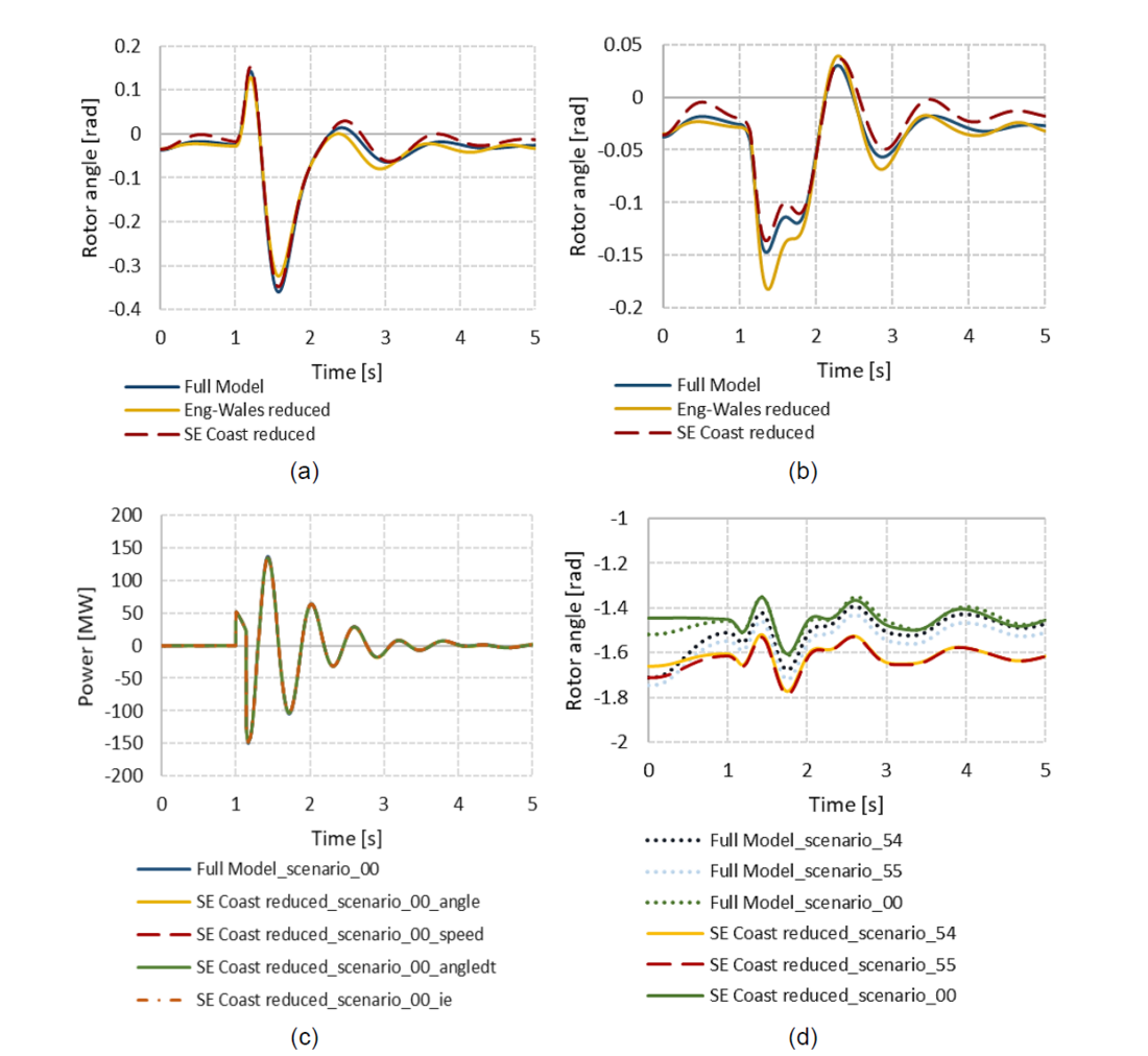
Figure 1 - Performance comparison of the dynamic equivalent network reduction technique
3.3. Machine learning classifier
Power system stability analysis is computationally expensive because of the small integration step sizes required to solve the differential equations defining the dynamics of the system. Machine Learning (ML) models offer an alternative way of capturing these dynamics with the help of data available from prior simulations. This approach is called supervised learning in ML parlance where the model relies on learning the non-linear functions with the help of training data. The advantage of this approach is that costly integration steps can be avoided completely which is particularly attractive when thousands of dynamic simulations need to be studied.
In this project, we have formulated the rotor angle stability analysis as a binary classification problem with the objective to categorise a set of inputs (known as features in ML) to a specific class. The features are the samples or scenarios of the system (a certain demand and dispatch level) and the class refers to the stable/unstable outcome of the system response.
There are several ML algorithms with slightly different approaches to identifying patterns in data such as gradient descent-based algorithms, distance-based algorithms, tree- based algorithms etc. In this project, we have considered three different types of classifiers, Support Vector Machines (SVC) [8], Gaussian Process Classifier (GPC) [9], and Random Forest Classifier (RFC) [10] and compared the performance to identify any specific advantages of a particular algorithm in relation to our dataset.
3.4. Active learning
To train a ML model, adequate training data are required to accurately capture the complex relationship among features and the target classes. For a complex problem like stability analysis of NETS, the number of dimensions of the feature space is extremely high and the performance of the ML model depends to a large extent on the quality of the samples. In this case, we have explored a special case of machine learning called Active Learning (AL) [11], to efficiently select the most useful observations which we can improve the model’s performance. This method has been previously used in power systems for dynamic security assessment and control [12]. The overall idea of the AL process is shown in Figure 2. The AL algorithm uses different sampling techniques to query a batch of samples from the unlabelled dataset (Pool set) to select the samples which are most effective in improving the probability of prediction of the stability outcome.
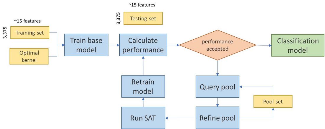
Figure 2 - Overview of the Active Learning process (part of SCT)
4. Stability assessment framework
The overall framework is split into two parts, the Stability Automation Tool (SAT) and Stability Classification Tool (SCT). SAT includes all the automation features discussed in Section 3.1 and the approach is generic enough to be used with network model of any sizes. To ensure efficient import/export of data, extensive use of local and cloud database systems have been used. This reduces the query times for large networks such as GB NETS.
SCT is an extension to the automation tool and users can use these tools independently or together depending on the requirement. Once the ML model is trained, it is specific to a particular boundary and the AL will no longer need to query points through the SAT. This holds true so long as there are no major topological changes to the network in future years as otherwise it would necessitate retraining the ML model.
4.1. Machine learning model
The machine learning (ML) model in SCT requires several data pre-processing steps to extract useful features from the raw data and prevent the model from being too specific to the training dataset. Figure 3(a) shows the data wrangling step which involves cleaning (removing any missing data), structuring and enriching (adding features from different sources) the raw data to form a master dataset which will then be passed on to the feature engineering step (Figure 3(b)).
There are several important steps in feature engineering such as scaling, binning, dimension reduction, feature selection with the final objective to identify a subset of most influential features which will have the maximum contribution towards increasing the accuracy of the model. These steps are discussed further in the following section.
In addition to the features, other factors which have significant influence on the performance of a classifier are the hyperparameters. These define the characteristics of the mathematical function behind a classifier algorithm. Once the dataset is finalised, a certain proportion of the data is used for hyperparameter optimisation. Different approaches are available to achieve this such as exhaustive grid search, Bayesian optimisation etc. A performance comparison of different techniques specific to our dataset is included in the results section of the paper.
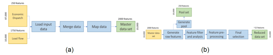
Figure 3 - Input data processing (a) data wrangling, (b) feature engineering
4.2. Feature engineering
A classification problem is heavily affected by the quality of its inputs such that relationships are uncovered among the most explanatory features. Feature engineering leverages data to create informative variables that are not there in the original raw dataset which exhibit a stronger relationship with the target outcome. Three main considerations have informed our approach to feature engineering; (i) feature generation to maximise explanatory power and concision of the feature set; (ii) feature analysis to enrich the data and avoid redundant information; and (iii) feature selection to maximise recovered variance from the master feature set while minimising the number of features to generalise the problem. Based on these, the following six steps have been implemented in the feature engineering part of the tool -
-
Generate features: These include demand and generation dispatch scenarios from a market simulator, load flow results such as transmission line flows and busbar voltages and angles, internal angle of synchronous machines etc. Additional features are derived to extract meaningful relationships such as asynchronous penetration in each zone of the 36-zone GB model.
- Filter features: Features which provide little information given by low (or zero) variance, are removed. Features with missing values are replaced by their respective means and removed if deemed appropriate by the variance filter.
-
Filter observations: Observations holding extreme values may skew the performance of classification methods which depend on feature scaling such as SVC. Deviations from common clustering are omitted from feature sets using isolation forests [13], which work well with high dimensional problems.
- Scale data: Gradient descent-based classifiers such as SVC require scaling of feature sets to avoid vastly different numeric ranges for different feature types. As an example, the range of values for line flows will be very different from internal angle of machines.
-
Reduce feature dimension: non-linear dimensionality reduction using manifold learning [14].
-
Select most explanatory features: Gradient boosting classifier builds an additive model in a forward stage-wise fashion; it allows for the optimization of arbitrary differentiable loss functions. In each stage, regression trees are fit on the negative gradient of the binomial or multinomial loss function. This provides an importance number associated with each feature which can be used to filter out features which are most influential.
Figure 4(a) shows the normalised importance measure of each of the top 60 features. Features at the top of the list have higher importance (broader base) i.e., more useful in terms of informing a classifier to predict the correct class. Names of all 60 features are not included in the figure, only a few are shown for reference. Figure 4(b) shows the cumulative importance of the top 60 features. All features after 54 have limited influence on the overall importance and they are excluded from the training set.
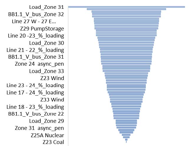
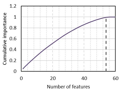
Figure 4 - Importance of top 60 features; (a) normalised importance of each feature, (b) cumulative importance
5. Results discussion
The performance of the machine learning model is discussed in terms of three points, (a) the size of the network, (b) classifier types and feature selection methods and (c) query strategy. A total of 18k scenarios have been used for the studies with a 70:30 split for training and testing.
5.1. Comparison of network sizes
To improve on the simulation time, the southeast coast of the 36-zone model is reduced to a dynamic equivalent. As discussed in Section 3.2, the dynamic responses of the reduced and the full model match quite well. Figure 5 shows the performance of the two models in terms of accurately identifying unstable operations when stepping through each iteration of the AL module. Only RFC results are shown here for the comparison with forward feature selection without any boosting [15] and undersampling [16]. The results show that reducing a part of the network far away from the boundary under study has no negative impact on the accuracy and it can be used to benefit from the improved simulation time. Therefore, for further comparison and analysis only the reduced network is used.
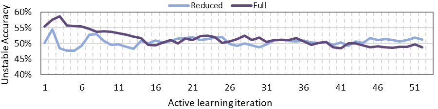
Figure 5 - Comparison of full and reduced 36-zone model performance
5.2. Comparison of machine learning classifier types
As discussed in Section 3.3, three different classifiers are explored in this work. Figure 6 presents a comparison in terms of the accuracy in identifying the unstable response of the system. Two different feature selection methods are considered, (a) forward selection and (b) gradient boosting. In addition, to avoid a bias towards the majority class (stable response in our case), adaptive boosting and undersampling techniques have been used. RFC is found to have the best performance with gradient boosting feature selection method and without adaptive boosting or undersampling.
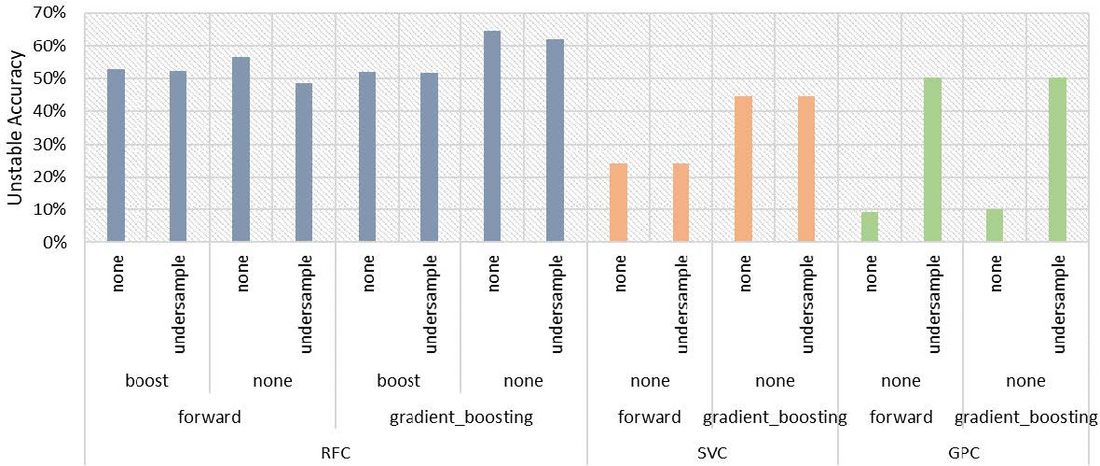
Figure 6 - Comparison of different classifier performance considering feature selection, boosting, and balancing
5.3. Comparison of query strategies
The active learning module queries a pool of unlabelled data (stable/unstable not known) to identify better the boundary between stable and unstable operational scenarios and in turn improves the accuracy of prediction. The objective is to query the most useful scenarios so that the accuracy improves in least number of iterations. The query strategy can be based on different measures of usefulness. Classification uncertainty is one such measure used in this case and compared with random sampling (no strategy). Figure 7 shows that random sampling performs much better than uncertainty measure (without adaptive boosting and undersampling). Since uncertainty is calculated for the most likely class, if the input data has imbalance of classes (more stable scenarios) then the query strategy tends to be biased towards a particular set of scenarios. Therefore, if the dataset is not well balanced, which is the most likely case for a real system, then random sampling can provide better accuracy for the minority (unstable scenarios) class prediction.
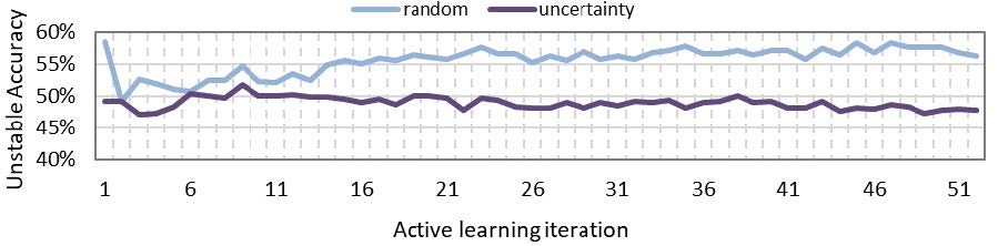
Figure 7 - Effect of query strategy on machine learning model accuracy
6. Conclusion
Stability analysis for year-round boundary capability assessment will be increasingly important for system operators around the world. The presence of uncertainties and variabilities in the input data in the planning timescale means a probabilistic approach is more suitable. However, there are several challenges in implementing a probabilistic framework for stability studies that need to be addressed thoroughly before such a tool can be used for business as usual (BAU). The framework proposed here shows that a combination of traditional analysis methods and techniques borrowed from other domains such as statistics and machine learning can be used to perform a year-round analysis in a real system. The initial results are promising but require further development to come up with a more succinct set of features that can improve the accuracy of the trained models further. Similar research from Imperial College London [17] shows that machine learning based approaches are promising in solving boundary capability studies. Such tools are expected to provide deeper insights into the system behaviour under changing generation mix and support the decision-making process in long-term planning and investments for reinforcements. The next step in the project is already underway to implement the framework with the ETYS model and we have managed to improve the accuracy further to 90%. The results will be compared with the ongoing planning cycles to assess the performance, suitability, and confidence in the approach before being adopted as a BAU tool.
References
- ‘Probabilistic planning for stability constraints’, https://www.smarternetworks.org/project/nia_ngso0036.
- ‘Network Options Assessment (NOA)’, https://www.nationalgrideso.com/research-publications/network-options-assessment-noa.
- ‘ETYS and Network Planning Process’ https://www.nationalgrideso.com/research-publications/etys/etys-and-the-network-planning-process
- R. Preece and J. V. Milanovic, “Assessing the Applicability of Uncertainty Importance Measures for Power System Studies,” IEEE Trans. Power Syst., vol. 31, no. 3, pp. 2076–2084, 2016, doi: 10.1109/TPWRS.2015.2449082.
- ‘Security and Quality of Supply Standard (SQSS)’, https://www.nationalgrideso.com/industry-information/codes/security-and-quality-supply-standards
- H. Urdal, R. Ierna, J. Zhu, C. Ivanov, A. Dahresobh and D. Rostom, "System strength considerations in a converter dominated power system," IET Renewable Power Generation, Vols. vol. 9, no. 1, pp. pp. 10-17, 2015.
- D. Chakravorty, B. Chaudhuri and S. Y. R. Hui, "Rapid Frequency Response From Smart Loads in Great Britain Power System," IEEE Transactions on Smart Grid, Vols. vol. 8, no. 5, pp. pp. 2160-2169, Sept. 2017.
- S. Abe, Support Vector Machines for Pattern Classification. London, England: Springer, 2012.
- C. E. Rasmussen and C. K. I. Williams, Gaussian processes for machine learning. London, England: MIT Press, 2019.
- R. G. McClarren, “Decision trees and random forests for regression and classification,” in Machine Learning for Engineers, Cham: Springer International Publishing, 2021, pp. 55–82.
- “modAL: A modular active learning framework for Python3 — modAL documentation,” Readthedocs.io. [Online]. Available: https://modal-python.readthedocs.io/en/latest/. [Accessed: 25-Oct-2021].
- “Data-Driven Security Rules for Real-time System Prediction and Control”, [Online]. Available: https://imperialcollegelondon.app.box.com/s/mhspl7hnsj4jgvfj8j0r6971z6qlsu48. [Accessed: 25-Oct-2021].
- Liu, Fei Tony & Ting, Kai & Zhou, Zhi-Hua. (2009). Isolation Forest. 413 - 422. 10.1109/ICDM.2008.17.
- Delicado, Pedro & Pachon-Garcia, Cristian. (2020). Multidimensional Scaling for Big Data
- “A Comprehensive Guide to Machine Learning”, [Online]. Available: https://snasiriany.me/files/ml-book.pdf [Accessed: 25-Oct-2021].
- H. He and E. A. Garcia, "Learning from Imbalanced Data," in IEEE Transactions on Knowledge and Data Engineering, vol. 21, no. 9, pp. 1263-1284, Sept. 2009, doi: 10.1109/TKDE.2008.239.
- Jochen L. Cremer, Goran Strbac, “A machine-learning based probabilistic perspective on dynamic security assessment,” International Journal of Electrical Power & Energy Systems, Volume 128, 2021, 106571, ISSN 0142-0615, https://doi.org/10.1016/j.ijepes.2020.106571.