Applied SARIMA Models for Forecasting Electricity Distribution Purchases and Sales
AUTHORS
U. MINNAAR - Research Testing and Development, Eskom Holdings SOC Ltd, Cape Town, South Africa
M. VAN ZYL, M. HICKS - Pricing and Sales, Eskom Holdings SOC Ltd, Cape Town, South Africa

Summary
South Africa’s power system is undergoing significant change as it simultaneously introduces renewable generation and unbundles the vertically integrated national utility, Eskom. Load forecasts play an important role in power system operation, and these changes increase the value of short- and medium-term forecasts for electricity distribution. This paper addresses the issue of short- and medium-term forecasting of electricity distribution wholesale purchases and sales by the development of SARIMA models. Models are presented for forecasting daily, weekly and monthly wholesale purchases as well as sales to large power users. Furthermore, the comparative performance of the SARIMA models is measured against naïve, LSTM and ARIMA forecasts. Forecasting performance is measured using MAPE and it is shown that the SARIMA models produce the best forecasting accuracy across the forecasting periods.
The development of models for the South African distribution sector is discussed along with the implementation and integration of the SARIMA forecasts within a web-based operational dashboard at the Distribution division of the national electricity utility, Eskom.
keywords
Electricity forecasting - SARIMA - time series forecasting1. Introduction
The ability to forecast electricity load is an important aspect of power system operation and is used for operational and financial management of utility operations across generation as well as transmission and distribution grids. It plays an important role in day-to-day operations, production planning, economic dispatch and unit commitment [1]. The introduction of Distributed Energy Resources (DER) such as renewable solar PV and wind energy as well as demand response means that it is important for utilities to match supply and demand on the power system across various time scales, from instantaneous up to several years [2].
Daily purchase and sales forecasts provide an important input to operational supply and demand balancing, as well as financial management of the utility. Furthermore, they are an important input into the management of electricity losses - particularly non-technical losses.
This paper discusses the development and application of Box-Jenkins Seasonal Autoregressive Integrated Moving Average (SARIMA) models for short- to medium-term (one day, one week and one month-ahead) forecasting of electricity purchases and sales for electricity distribution in South Africa, as well as the operational implementation of the forecasts within a utility dashboard for data access and visualization.
2. Value of load forecasting to utilities
The operation of a power system typically requires reacting to the load requirements of grid connected customers. For this reason, load forecasting plays a critical role in any electricity utility as it allows for the utility to respond to changing load requirements. Prior knowledge of available generation and load requirements are critical to ensure that no generation shortages occur [3].
The quality of a demand forecast has a direct effect on the economic viability and reliability of an electricity utility. Important utility operating decisions are reliant on an accurate demand forecast, including: scheduling of power generation and fuel purchasing, scheduling of maintenance, designing rate structures, financial planning and planning of energy transactions [2] [3] [4].
The importance of accurate load forecasts is further highlighted in [5], where the volatility of renewable energy plants is evaluated. This, in combination with increased renewable energy penetration in electricity markets, emphasizes the need for accurate load forecasts to assist in planning of dispatch [2] [5].
In [2], the dangers of inaccurate load forecasts are highlighted. Inaccurate load forecasts may lead to a significant financial burden- in some cases even bankruptcy - of an electricity utility. Since load forecasts are also typically used for system maintenance and planning, inaccurate forecasts may also lead to a critical shortage of generation capacity, which in turn could lead to equipment failure or, in a worst-case scenario, a system-wide blackout. In the South African context, the importance of forecasts was demonstrated by the prediction of the 1998 White Paper on Energy, which stated that the country would require additional generation capacity by 2007 [6]. South Africa failed to add the required generation capacity and experienced the first round of load shedding the following year, 2008, with load shedding having occurred regularly since [6].
3. Forecasting Applications
The factors that influence load forecast accuracy are also analyzed in [2], these include but are not limited to: geographic diversity (assuming geographic data is used in the forecast), data quality, forecast horizon (forecast time period), forecast origin and customer/data segmentation or aggregation [2].
3.1. Types of Forecasting
It is recommended by Hong [2], that long term forecasts remain probabilistic in nature rather than forecasting a single point. This stems from the fact that no forecast is 100% accurate and while these errors are small for shorter forecast horizons, errors become more prevalent as the forecast horizon increases. Doing a probabilistic forecast assists utilities in planning for worst- and best-case scenarios, and significantly decreases the likelihood that the utility is caught unaware [2]. Kyriakides and Polycarpou [3] separate load forecasting into two different categories, namely classical or computational intelligence-based (machine learning) approaches. Some of the techniques associated with these approaches to forecasting are presented in Table 1.
| Approach | Techniques |
|---|---|
Conventional / Classical | Time Series models |
Regression models | |
Kalman filtering based techniques | |
Machine Learning | Artificial Neural Networks (ANN) |
Expert Systems | |
Fuzzy-inference and fuzzy-neural models | |
Evolutionary programming and genetic algorithms | |
Support Vector Machines (SVM) | |
Multi-layer Perceptron (MLP) | |
Long Short-Term Memory neural network (LSTM) | |
Recurrent Neural Network (RNN) |
Makridakis et al. have shown that despite significant development in the field of machine learning forecasting techniques, statistical forecasting techniques retain higher levels of accuracy [7]. In addition, machine learning techniques have the disadvantage of higher computing complexity and computational execution time when compared to classical statistical techniques [7].
Another key disadvantage of machine learning techniques (e.g. artificial neural networks) is their black-box nature, which in practice gives poor explanations of the non-linear functions found in the time series results [8].
3.2. Forecasting time horizons
Electric load forecasting is typically broken up into three different time horizon categories [3] that meet differing utility operational and business needs. These are Short- (STLF), Medium- (MTLF) and Long-Term Load Forecasting (LTLF). Very Short-Term Load Forecasting (VSTLF) is also highlighted as a forecast timeline that looks from a few minutes ahead up to several hours [5]. Each of these forecasting timelines are summarized in Table 2 below.
| Forecasting Timeline | Period | Function |
|---|---|---|
Very Short-Term Load Forecasting (VSTLF) [5]
| Minutes up to a few hours ahead[2] Up to 1 hour-ahead[5] | Power plant management and planning. Provisioning of ancillary services such as regulation frequency control and ramping capacity
|
Short Term Load Forecasting (STLF)[3] [5] | 1 day- to 1 week-ahead[2] 1 hour- to 1-week-ahead[3] 1 day-ahead [5] | Used in day-to-day operations. Scheduling of start-up times. Load flow analysis. Power system security studies. |
Medium Term Load Forecasting (MTLF)[3][5] | 2 weeks- to 3 years-ahead[2] 1 week- to 1 year-ahead[3] Up to 1 month-ahead [5] | Scheduling maintenance and fuel supply. Minor infrastructure adjustments/improvements. |
Long Term Load Forecasting (LTLF)[3] [5] | 3 years- to 50 years-ahead[2] >1 year-ahead[5] | Planning of construction of new power stations or grid expansion. General increases to the transmission system capacity. Expansion planning |
Referring to Table 2, a focus will primarily be placed on STLF and MTLF, as their associated functions meet the typical requirements of an electricity utility at the Distribution level. STLF is particularly critical in every electricity utility’s operation as it provides the necessary input data for load flow studies and contingency analysis done by the utility. These studies form the basis for the utilities’ planning decisions, such as Transmission purchase volumes (in an unbundled utility) or to determine grid constraints in advance [3]. While such applications are often focused on total demand over a specified period, variations can also be developed to meet differing needs of power system operations e.g. predicting the times and volumes of maximum and minimum system demand.
In contrast, LTLF would typically be associated with Generation and Transmission processes for purposes of expansion planning, while VSTLF is associated with the System Operator, where the granularity of the forecast is optimal for generation unit commitment on a merit-order basis. VSTLF is also widely used in the forecasting of renewable energy output, where the primarily weather-related input variables (e.g. solar irradiation and wind velocity) can be extremely volatile and must therefore be updated frequently as more reliable input data is made available. Such forecasts typically rely on input data from 3rd party sources (e.g. a weather service) and provision must be made for the data to be refreshed at an interval suitable to the forecasting application. Since input parameters to VSTLF models tend to be volatile, and forecasting accuracy decreases substantially the further ahead one attempts to predict, VSTLF models are unsuitable for implementation in applications where predictions are required greater than a few hours ahead.
4. The South African Electricity Landscape
At the time of writing, South Africa has a largely vertically integrated electricity structure with the national utility, Eskom, responsible for the bulk of electricity generation alongside independent power producers (IPPs), as well as owning and operating the transmission network. Distribution is split between Eskom and municipalities (redistributors), with Eskom supplying ~40% of distribution customers in the country and the remaining (~60%) supplied by ~180 local municipalities [9].
In 2019 the South African president announced the unbundling of Eskom, and this process has kick-started power sector reform in the country. Following this, the Department of Public Enterprises released a roadmap for the restructuring of Eskom in 2019 [10], which outlines the unbundling and legal separation of Eskom as a vertically integrated utility, as well as articulating a number of policy statements regarding the Electricity Supply Industry in South Africa. The current structure of the South African electricity sector is presented graphically in Figure 1.
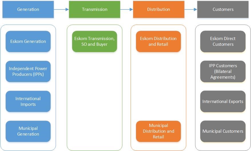
Figure 1 - Structure of the South African Electricity Sector [9]
The restructuring of the national utility increases the importance of accurate forecasts for the Distribution division for financial and management planning of the Distribution company as it stands financially independent from the Transmission wholesaler.
Alongside the structural changes to the electricity supply industry, other industry developments related to the regulatory environment and renewable energy increase the importance and value of short-term forecasting of electrical purchases and sales for the distribution utility.
The first is the continuing growth in renewable generation associated with the country’s Renewable Energy Integrated Power Purchase Program (REIPPP). This has seen the installation of more than 6806 MW [11] of solar PV and wind generation across four bid windows, with more bid windows due to be released. Alongside this, the ongoing presence of load shedding due to a shortfall in generation capacity has encouraged significant growth in small scale solar generation as well as energy storage within the small-scale generation market.
The second is the amendment to Schedule 2 of the country’s Electricity Regulation Act [12] exempting generation facilities below 100 MW from requiring a generating license, with the aim of shortening the regulatory processes for new generation and encouraging private sector investment in electricity generation. A consequence of this is likely to be further acceleration of renewable generation, either as self-generation at large industrial or mining customers or the development of new generation facilities linked to power purchase agreements with customers where electricity is wheeled across the transmission and distribution grids. The country’s mining industry has already indicated that they have 3900 MW of renewable solar, wind and battery energy projects in various stages of development [13].
The value of self-generation as a price hedge for mining customers has been explained by Minerals Council CEO, Roger Baxter, who stated “Solar has a design life of 25 years. If it gives you 10% or 5% of your energy needs, you can hedge the cost for 20 years. You won’t have any cost increases. Effectively, you’ll be doing that at the level of inflation…” [14].
The growth in renewables, both at utility-scale as well as embedded generators, affects the supply and demand balance. Accurate load forecasts become an increasingly important tool for utilities for both financial and operational management in this environment.
Electricity Purchases and Sales in South Africa
Eskom’s distribution network consists of ~358,100 km of medium and high voltage overhead lines and cables ranging from 1kV to 132kV, with 155,623 MVA transformer capacity supplying 6,857,018 customers [15]. These customers are broadly categorized as either Large Power User (LPU), Small Power User (SPU) or Pre-Paid User (PPU) type consumers.
The designation of a customer as either an LPU, SPU or PPU is based on several technical factors – including the supply voltage, load factor and notified maximum demand (NMD) of the customer. In general, LPU customers are those with a high load factor, high demand characteristics (i.e., large industrial and commercial consumers), while SPU customers are those with low load factor, low demand characteristics (i.e., predominantly residential consumers, with a small percentage of small commercial and industrial customers). PPU customers share identical characteristics to their SPU counterparts, however the customers purchase electricity tokens in advance of their consumption, rather than receiving a monthly bill.
Time-of-Use (TOU) tariffs are applied for LPU customers as a means of balancing the national demand. To this end, each hour of each day is designated as either a Peak, Standard or Off-Peak consumption block. The tariff structure for LPU customers incentivizes customers to reduce their consumption during Peak hours by applying increased energy charges, and decreasing charges for Standard and Off-Peak hours, respectively. To facilitate this billing process, Eskom employs interval metering for all customers on LPU tariffs, whereby consumption is recorded on a half-hourly basis and transmitted to Eskom data servers for processing and billing.
Table 3 summarizes the differences between the three customer categories.
| Large Power Users (LPU) | Small Power Users (SPU) | Prepaid Power Users (PPU) |
|---|---|---|
Redistributors, large industrial, commercial and mining | Small industrial, agricultural commercial and residential | Residential |
High load factor | Low load factor | Low load factor |
High NMD | Low NMD (less than 100kVa) | Low NMD (less than 100kVa) |
Supply voltage from < 500V up to 132kV (or may be transmission-connected). | Supply voltage < 500V. | Supply voltage < 500V. |
Seasonally and time-of-use differentiated tariffs. | Non-differentiated, inclining block rate tariffs. | Non-differentiated, inclining block rate tariffs. |
30-minute Interval Metering | Post-paid monthly metering or estimation | Pre-paid token purchases. |
A significant majority of Eskom’s Distribution customers are residential customers with pre-payment meters, which comprise ~95% of customers but only constitute ~4% of electricity sales by the utility. Table 4 illustrates that while residential prepaid customers make up the vast majority of customers, they consume only a small share of electricity sales.
The remaining customer base and associated energy sales are attributed to Large Power Users and Key Industrial Customers.
| Customer Class | Number of Customers | Percentage of Electricity Sales |
|---|---|---|
Large Power Users | 22534 | 9.7% |
Large Industrial & Commercial Customers | 586
| 34%
|
Municipalities | 177 | 44.9% |
Independent Power Producers | 127 | 0.1% |
Small Power Users | 321925 | 6.6% |
Prepaid | 6603663 | 4.7% |
TOTAL | 6949636 | 100% |
Electricity is purchased from the Transmission operator as well as from renewable independent power producers (IPPs) which are connected to both the transmission and distribution networks.
5. Existing Eskom Distribution Sales Forecasting Process
Historically, the primary objective of forecasting within Eskom Distribution has been to provide accurate forecasting of electricity sales for use in distribution network planning, as well as tariff design and revenue determination processes. These forecasts typically provide monthly kWh demand per TOU (Time-of-Use) block, as well as whether Notified Maximum Demand (NMD) will be exceeded.
The forecasts are presented in a monthly format for a period of 15 years and are updated annually. A “bottom-up” approach to forecasting is utilized, whereby forecasts are produced individually for larger customers, while smaller customers are grouped together. This allows the forecasters to follow a different process for each customer depending on the quantity and range of data available – for example, a forecaster may be aware that a particular customer has plans for expansion in the coming financial year; this will be used to inform the sales forecast. In general, all forecasts follow a process of deriving historical trends based on regression analysis, predicting future demand based on these trends, and adjusting based on specific and relevant customer information (e.g. expansion plans).
In contrast to the above, this paper investigates statistical forecasting methods for the Distribution environment. The existing forecasting method is manual and highly labour intensive. It also requires employees with significant knowledge of the local market and environment. Statistical methods, such as the SARIMA method discussed in this paper, present an opportunity to introduce less labour-intensive practices that are also suitable for automation of forecasting.
6. Purchases and Sales Data
The data used for this study comprises of the wholesale purchases that the Distribution utility purchases from Eskom’s Transmission subsidiary, international imports and renewable power producers, as well sales to large power user (LPU) customers for whom interval metered data is available and which dominate electricity distribution sales. Renewable generation comprises ~ 6% of electricity generated in South Africa [11]. In effect, the input data consists of South Africa’s total monthly electricity consumption. Since 2008 South Africa has experienced a generation capacity shortage which has resulted in rotating load shedding being implemented sporadically throughout the country.
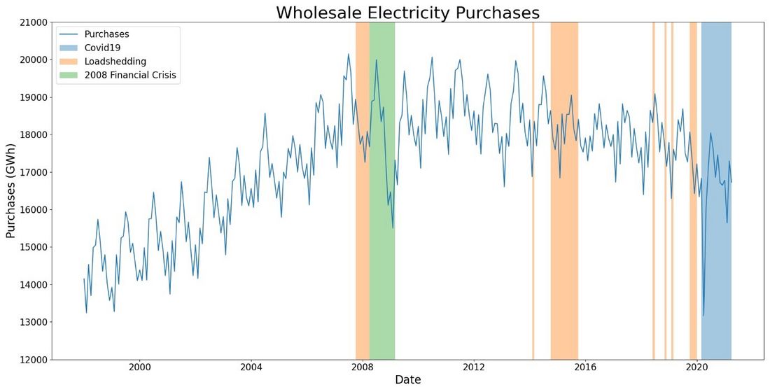
Figure 2 - Wholesale Electricity Purchases
Figure 2 illustrates the historical wholesale purchases from 1998-2021. Periods of load shedding occurrence are indicated, as well as the Covid-19 national state of disaster [16] effective from March 2020. Figure 2 illustrates monthly electricity wholesale purchases peaked in July 2007 at 20153 GWh, which includes a small number of large customers connected to the transmission grid.
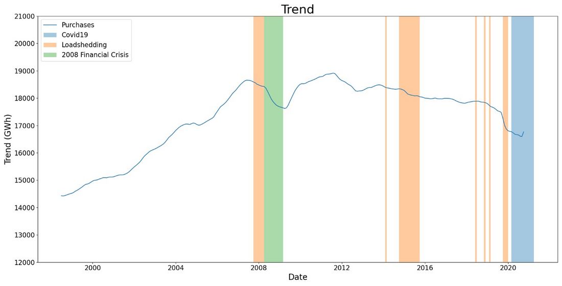
Figure 3 - Wholesale Distribution Purchases Trend
Figure 3 illustrates the long-term trend of the wholesale electricity purchases. The following trends can be seen:
- Electricity consumption in South Africa increased annually until 2007, when South Africa did not add the required generation capacity, and then remained approximately constant from 2009 until 2013. The extended period of increasing consumption prior to 2007 coincided with South Africa having adequate generation capacity and the lowest electricity prices in the world [6].
- From 2014 onwards electricity consumption has shown a declining trend due to generation supply constraints (which also encouraged additional activities e.g. growth in distributed energy generation, energy efficiency)
- The impact of the 2008 financial crisis and the 2020 COVID-19 national state of disaster can be clearly seen, with significant reductions in wholesale purchases in 2008 and 2020.
In time series analysis, seasonality refers to periodic fluctuations or repeating patterns over fixed periods [17]. Electricity consumption in South Africa exhibits these repeating patterns on multiple time scales (namely hourly, daily and monthly), as a result of human behavior as well as annual weather patterns. On an hourly basis, the daily demands cycle for electricity consumption in South Africa, clearly indicating distinct morning and evening peak periods. The same observation can be made for weekly electricity consumption with distinct and repeating daily peak sales in the middle of the week and lower consumption over weekends. The repeating patterns typical of seasonality are shown for hourly, daily and monthly electricity purchases (extracted via a seasonal decomposition) in Figure 4.
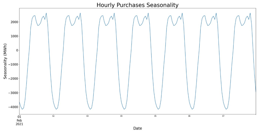
Figure 4 - Seasonality of Electricity Purchases
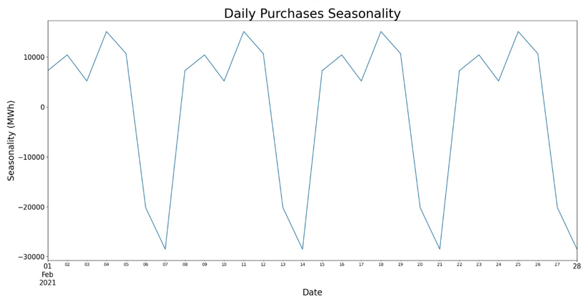
Figure 4 - Seasonality of Electricity Purchases
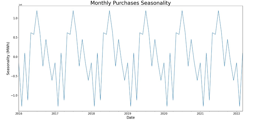
Figure 4 - Seasonality of Electricity Purchases
The impact of weather on electricity sales and demand is so distinct that the national utility, Eskom, defines seasonal peak and off-peak periods according to a high demand season from 1 June to 31 August over winter and a low demand season from 1 September to 31 May [18]. Power station maintenance is minimized during the high demand season in the winter months, with planning and implementation of power station maintenance being scheduled primarily during the lower demand summer months [19].
7. Selection of Forecasting algorithm
The Box-Jenkins Seasonal Auto Regressive Integrated Moving Average Model (SARIMA) was chosen as the forecasting model for implementation as it is a commonly used linear model, recognized as being highly effective. SARIMA has been applied across a wide range of applications for seasonal time series forecasting and has minimal data input requirements [8]. It has been shown to have high accuracy for datasets with seasonal variations, while being easy to implement.
Box-Jenkins SARIMA Model
The Seasonal Autoregressive Integrated Moving Average (SARIMA) model is a time series prediction model introduced by Box and Jenkins [20], that is widely used for time series forecasting in a wide range of applications, including: river water flows [21], inflation rates, infectious diseases [22], sea level variability [23] and electricity production and demand [1] [24]. The SARIMA (p, d, q) (P, D, Q)S model can be written as [20]:
where p is the non-seasonal AR order; d is the non-seasonal difference; q is the non-seasonal MA order; P is the seasonal AR order; D is the seasonal difference; Q is the seasonal MA order; and S is the time span of the repeating seasonal pattern.
The SARIMA model has been selected due to its successful application across a wide variety of applications, its suitability as a forecasting method for datasets with seasonality, as well as its autoregressive characteristics.

8. Parameter Selection
The selection of the seasonal (P, D, Q) and non-seasonal (p, d, q) parameters are chosen based on evaluating Akaike’s Information Criterion (AIC) of candidate models.
Information criteria techniques refer to model selection methods that are based on likelihood functions and are applied to parametric model-based problems [25].
Akaike’s Information Criterion is a mathematical model that estimates out-of-sample prediction error, and therefore the quality of a candidate model for a given dataset [25]. It estimates model quality relative to other models for the same dataset, thereby providing a means for model selection. The AIC of a particular forecasting model can be calculated as:
Where L is the likelihood under the fitted model and p is the number of parameters in the model.
Model selection is done by choosing the model with the minimum AIC out of the range of models considered.
Test forecasts have been conducted on a daily, weekly and monthly basis for wholesale purchases and the results are illustrated below. The same model selection and testing process is followed for LPU sales, and the accuracy performance is discussed alongside those for wholesale electricity purchases. The primary metric used to estimate the accuracy of the forecasts in this study is the Mean Absolute Percentage Error (MAPE), while Mean Absolute Error (MAE), and Root Mean Square Error (RMSE) of forecasts are also reported.
Forecasting accuracy performance results and graphs are discussed and analyzed for wholesale electricity purchases. A comparative analysis is conducted to benchmark the performance of the trained SARIMA models against naïve (persistence), ARIMA and LSTM forecasts and the performance metrics for LPU sales are discussed as part of the comparative performance analysis.
A SARIMA model was trained using daily wholesale purchases data for the period of January 2016 – June 2021. Daily and week-ahead forecasts were produced using the months from July to September as the test data. For the monthly data, the operational requirement is a month-ahead forecast and the initial training set is January 2016 – December 2017. A rolling month-ahead forecast is used for testing, with the SARIMA model updated monthly.
The top 3 models’ parameters for daily and monthly purchases with corresponding AIC scores are shown in Table 5 and Table 6 respectively.
| Non-seasonal Parameters (p, d, q) | Seasonal Parameters (P, D, Q, s) | AIC (MWh) |
|---|---|---|
| (1, 1, 1, 7) | 46472 |
| (2, 1, 1, 7) | 46601 |
| (2, 1, 1, 7) | 47003 |
| Non-seasonal Parameters (p, d, q) | Seasonal Parameters (P, D, Q, s) | AIC (GWh) |
|---|---|---|
| (0, 1, 0, 12) | 1746 |
| (0, 1, 0, 12) | 1756 |
| (0, 1, 2, 12) | 1760 |
Based on the AIC scores, a SARIMA (5,1,3) (1,1,1)7 and SARIMA (2,1,2) (0,1,2)12 model was selected for daily and monthly forecasting respectively.
9. Results
9.1. Daily and Weekly Wholesale Purchases
The results of a day-ahead rolling SARIMA forecast for wholesale purchases over a three-month testing period are shown in Figure 5, alongside rolling Persistence, ARIMA and LSTM models trained on the same dataset. These forecasts have been plotted against the observed values over the testing period in order to assess the relative accuracy of each model. The period selected for the rolling forecasts are the three months from 1 July to 30 September 2021. While a longer testing period may have been ideal, this window was selected as it coincided with a period where no load shedding was implemented, eliminating the possible impact of load shedding affecting the results.
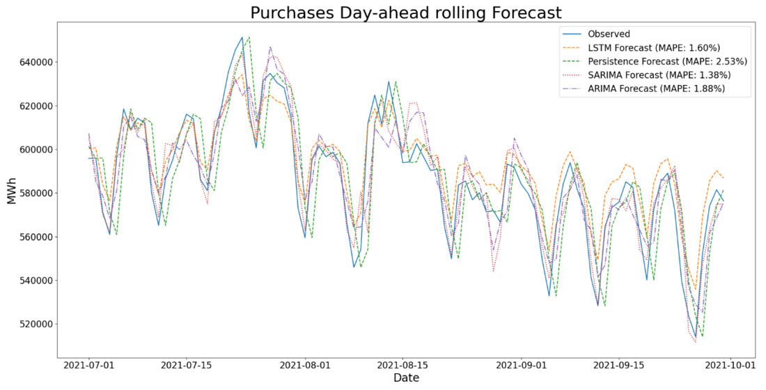
Figure 5 - Wholesale Electricity Purchases Day-ahead Rolling Forecast
The Persistence (naïve) model is the simplest forecasting model to implement in that it takes the current (observed) value and forecasts it for the next period. The model used in the above comparison forecasts the value for the period t+1 to be equal to the period before it (t), where t represents a time step in the relevant dataset. The Persistence model produced the lowest accuracy of all forecasting models considered, with a MAPE of 2.53% and MAE of 14839 MWh.
The parameters of the ARIMA model utilized in the above forecast are similar to the SARIMA model as previously discussed, however the seasonal components are removed. The model can be described as ARIMA (4,1,3). As a more sophisticated model, ARIMA produced greater accuracy than that of the persistence model, however its performance does not match other models which have been considered in this paper due to its lack of consideration for seasonal trends. ARIMA produced a MAPE of 1.88% and MAE of 10999MWh.
The Long Short-Term Memory model (LSTM) is a recurrent neural network machine learning model typically associated with forecasting time-series data. The model consists of distinct memory blocks, each with a selection of decision gates which can be represented mathematically. These gates can be manipulated by adjusting several different input parameters to the model. The look-back time increases the amount of data the model considers when making a forecast. The look-back time typically equates to the time horizon being forecasted for, in the case of a day-ahead forecast, the look back parameter was set to 1. Another parameter to be tuned is the number of layers in the model, which varies depending on the dataset characteristics. In this case, the optimal number of layers was found to be 2. LSTM produced a MAPE of 1.60% and MAE of 9365 MWh.
The comparative performance results for the day-ahead rolling forecast are summarized in Table 7. These forecast results indicate that the SARIMA (5,1,3) (1,1,1)7 model was the best performing model, with a MAPE of 1.38% and MAE of 8109MWh.
| Forecast Model | MAE (MWh) | MAPE (%) | RMSE (%) |
|---|---|---|---|
SARIMA (5,1,3) (1,1,1)7 | 8109 | 1.38 | 1.91 |
ARIMA (4,1,3) | 10999 | 1.88 | 2.24 |
LSTM | 9365 | 1.60 | 1.86 |
Persistence | 14839 | 2.53 | 3.22 |
9.2. Daily and Weekly LPU Sales
The models as described above for forecasting wholesale transmission purchases were also trained and applied to forecast LPU sales at a distribution level. This is because the datasets exhibit identical seasonal and historical trends due to their mathematical relationship, which can be described as:
LPU Sales = Transmission Purchases - Distribution Losses - (SPU Sales + PPU Sales)
As with the wholesale transmission purchases above, the models have been trained on historical LPU Sales data and rolling forecasts have been generated for the testing period 1 July to 30 September 2021. These forecasts are plotted against the observed values in Figure 6 below.
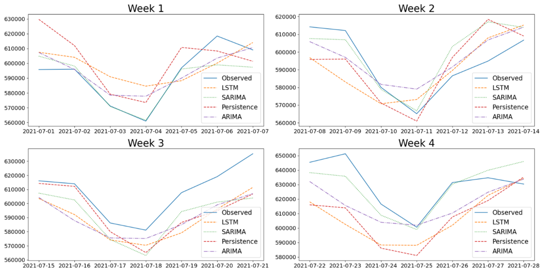
Figure 6 - Electricity week-ahead forecast
Table 8 shows the average MAPE, MAE and RMSE for the 12 week-ahead forecasts generated over the testing period. As with the purchases dataset, SARIMA proved to be the best performing model with a MAPE of 2.63% and MAE of 15361 MWh.
| Forecast Model | MAE (MWh) | MAPE (%) | RMSE (%) |
|---|---|---|---|
SARIMA (5,1,3) (1,1,1)7 | 15361 | 2.63 | 3.00 |
ARIMA (4,1,3) | 15620 | 2.67 | 3.03 |
LSTM | 21832 | 3.72 | 4.30 |
Persistence | 18921 | 3.22 | 3.66 |
9.3. Monthly Wholesale Purchases
Monthly forecasts are evaluated based on a rolling month-ahead forecast running from January 2018 until December 2021. The results for the month-ahead rolling forecast for wholesale purchases is shown in Figure 7 alongside the observed values and rolling forecasts from Persistence, ARIMA and LSTM models trained on the same dataset.
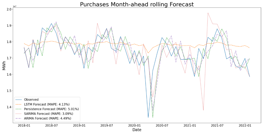
Figure 7 - Purchases month-ahead rolling forecast comparison
As with the daily and weekly forecasts, the SARIMA (2,1,2) (0,1,0)12 is the best performing model in the comparative benchmark, producing a MAPE of 3.09% against 4.13%, 4.49% and 5.01% for LSTM, ARIMA and Persistence models, respectively. The results are summarized in Table 9.
| Forecast Model | MAPE (%) | MAE (MWh) | RMSE (%) |
|---|---|---|---|
SARIMA (2,1,2) (0,1,0) 12 | 3.09 | 537912 | 5.02 |
ARIMA (2,1,2) | 4.49 | 782715 | 5.86 |
LSTM | 4.13 | 718754 | 5.51 |
Persistence | 5.01 | 872634 | 6.29 |
9.4. Monthly LPU Sales
The training and testing process for monthly wholesale purchases was replicated for monthly LPU sales, and the results were similar, with SARIMA (3,1,2) (1,1,1)12 proving to be the best performing model.
9.5. Results
From the models which have been evaluated for forecasting electricity wholesale purchases and sales, SARIMA models are shown to have the best performance across daily, weekly and monthly forecast windows for both purchases and sales. Table 10 shows MAPE and RMSE results for rolling day-ahead and week-ahead LPU sales forecasts alongside those for purchases, with Table 11 showing results for the monthly forecasts.
Parameter | Model | Rolling Day-Ahead | Week Ahead | ||
MAPE (%) | RMSE (%) | MAPE (%) | RMSE (%) | ||
Purchases | SARIMA (5,1,3) (1,1,1)7 | 1.38 | 1.91 | 2.63 | 3.00 |
ARIMA (4,1,3) | 1.876 | 2.24 | 2.67 | 3.03 | |
LSTM | 1.597 | 1.86 | 3.72 | 4.30 | |
Persistence | 2.53 | 3.22 | 3.22 | 3.66 | |
LPU Sales
| SARIMA (3,1,3) (2,1,1)7 | 0.97 | 1.44 | 1.54 | 1.78 |
ARIMA (3,1,3) | 2.07 | 2.53 | 2.02 | 2.35 | |
LSTM | 1.62 | 1.88 | 2.71 | 3.16 | |
Persistence | 2.32 | 3.04 | 1.85 | 2.20 | |
Parameter | Model | Rolling Month-Ahead | |
MAPE (%) | RMSE (%) | ||
Purchases | SARIMA (2,1,2) (0,1,0)12 | 3.09 | 5.02 |
ARIMA (2,1,2) | 4.49 | 5.86 | |
LSTM | 4.13 | 5.51 | |
Persistence | 5.01 | 6.29 | |
LPU Sales
| SARIMA (3,1,2) (1,1,1)12 | 3.48 | 5.75 |
ARIMA (3,1,2) | 4.36 | 5.87 | |
LSTM | 3.49 | 4.97 | |
Persistence | 5.13 | 6.55 | |
Table 10 and Table 11 show that the forecasting performance of the SARIMA models perform similarly across the forecasting timeframes for both sales and purchases. The SARIMA models have the best forecasting performance when benchmarked against Persistence, LSTM and ARIMA models.
10. Application within a Utility Sales and Purchases Dashboard
A platform for sharing electricity sales and purchases forecast data was developed to support operational monitoring and analysis as well as provide inputs to regulatory tariff applications and engagements. To facilitate this, an interactive browser-based Dashboard was developed using the Python programming language alongside the Plotly Dash web development framework.
The aim of the dashboard is twofold - firstly, it provides a centralized platform for easy access to daily sales data. The dashboard provides access to the underlying sales and customer databases and datasets can be drawn and configured in various structures and time scales e.g. tariff structures, network areas, provincially etc. The dashboard allows a user to query, display and download historical and forecast electricity sales and purchases values.
The second aspect is that sales and purchases forecasts are displayed for both day and week-ahead periods and are, along with month-ahead forecasts, integrated into system calculations to estimate daily sales for PPU and SPU customers as well as estimating daily losses incurred by the utility. The SARIMA models developed in this paper are applied within this operational dashboard.
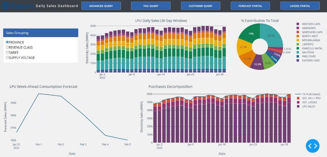
Figure 8 - Utility dashboard landing page
Figure 8 shows the landing page of the dashboard, which gives the users a view of the sales breakdown, and can be configured according to province, revenues class, tariff or supply voltage. The landing page also provides a sales forecast for LPU customers alongside a breakdown of overall purchases broken down by LPU sales alongside estimations of losses and SPU/PPU sales.
The dashboard further assists business operations by incorporating built-in Time of Use analysis on both a National and individual customer level. This allows users to monitor how individual customers as well as categories of customers react to time-of-use pricing signals. Figure 9 illustrates the Time-of-Use page, which provides data for the high and low demand seasons.
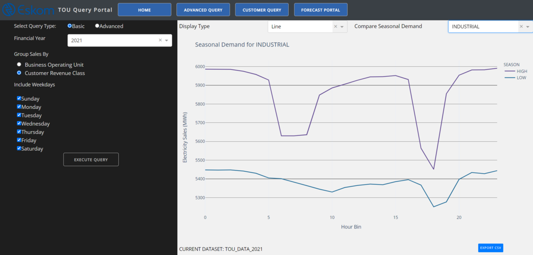
Figure 9 - Time of Use Page
Finally, the dashboard provides detailed metrics to provide users with transparent information as to the accuracy of the Sales and Purchases forecasts which have been developed. Users can directly compare forecast sales and purchases values against historical actual values and export these values for further analysis. Figure 10 shows the forecast page with actual LPU sales plotted as a bar plot against the forecast for a particular day. Daily forecasts are scheduled for a week-ahead and the actual sales and forecast values are made available for download to the end-user.
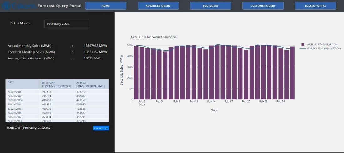
Figure 10 - Forecast Page
The SARIMA forecast implemented within the dashboard is modified to account for reduced sales on public holidays as well as school holidays. This improves the SARIMA forecast accuracy for the week ahead forecast to 1.72% from 2.63%.
11. Conclusions
South Africa’s power system is undergoing significant changes as it simultaneously introduces renewable generation and unbundles the national utility, Eskom. In this changing environment load forecasts play a significant role in both the operational and financial management of the separated utility functions. In this study, seasonal autoregressive integrated moving average (SARIMA) models have been developed for short- to medium-term load forecasting applications, namely day- ahead, week-ahead and monthly forecasts. The SARIMA models’ performance is benchmarked against naïve, LSTM and ARIMA models. The comparative benchmark results show that the SARIMA forecast models have the highest forecasting accuracy for all three forecast scenarios.
A distribution utility dashboard has been developed to enable easy access to sales and forecasting data, and the SARIMA models are applied for operational forecasts within this dashboard.
Future Work
Future development of the implemented model will focus on the addition of weather data, specifically temperature data, as an input parameter to improve forecast accuracy. Additionally, the implemented model forecast accuracy is impacted by South Africa’s generation shortfall and the consequent load shedding implemented by the system operator. Methods to compensate for the impact of load shedding on forecast accuracy will be developed and tested. The restructuring of Eskom into functionally separated entities will also see the introduction of a day-ahead energy market. Future forecasting initiatives include the development of hourly load forecasting models to meet the needs of the energy market.
References
- O. Bozkurt, G. Biricik and Z. Taysi, "Artificial neural network and SARIMA based models for power load forecasting in turkish electricity market," PLOS ONE, vol. 12, no. 4, 2017.
- T. Hong, C. Shahidehpour and Mohammad Shahidehpour, "Load Forecasting: Case Study," EISPC, Chicago, 2015.
- E. Kyriakides and M. Polycarpou, "Short Term Electric Load Forecasting: A Tutorial," Springer, Heidelberg, 2007.
- Z. Kong, Z. Xia, Y. Cui and H. Lv, "Probabilistic Forecasting of Short-Term Electric Load Demand: An Integration Scheme Based on Correlation Analysis and Improved Weighted Extreme Learning Machine," MDPI, Wuhan, China, 2019.
- L. Burg, G. Gürses-Tran, R. Madlener and A. Monti, "Comparative Analysis of Load Forecasting Models for Varying Time Horizons and Load Aggregation Levels," MDPI, Aachen, Germany, 2021.
- T. Ledger, "Why The Lights Went Out: Power Sector Reform In South Africa," Public Affiars Research Institute, Johannesburg, 2019.
- S. Makridakis, E. Spiliotis and V. Assimakopoulos, "Statistical and Machine Learning," PloS ONE, vol. 13, no. 3, 2018.
- M. Khashei and M. Bijari , "A novel hybridization of artificial neural networks and ARIMA models for time series forecasting," Applied Soft Computing, vol. 11, no. 2, pp. 2664-2675, 2011.
- E. Teljeur, S. Dasarath , F. Kolobe and T. Da Costa , "Electricity Supply Industry Restructuring: Options for the Organisation of Government Assets," Trade & Industrial Policy Strategies and Business Leadership, Pretoria, 2016.
- Department of Public Enterprises, "Roadmap for Eskom in a reformed Electricity Supply Industry," Public Enterprises, Pretoria, 2019.
- J. Wright and J. Calitz, "Statistics of utility-scale power generation in South Africa H1-2021," July 2021. [Online] [Accessed 16 April 2022].
- Department of Mineral Resources and Energy, "Amendment of Government Notice No. 737, Published on 12 August 2021,Government Gazette 44989: Licensing Exemption and Registration Notice," Government Gazette, 5 October 2021.
- Minerals Council South Africa, "Media Statement: Minerals Council Welcomes President's Announcementof increased embedded generation threshold to100MW," 23 November 2021 [Online] [Accessed 2022 March 04].
- T. Creamer, "EngineeringNews," 06 02 2020. [Online]
- Eskom , "Integrated Report," Eskom, Johannesburg, 2021.
- Department of Co-Operative Governance And Traditional Affairs, "Declaration of National State of Disaster," 15 March 2020. [Online] [Accessed 14 October 2021].
- National Institute of Standards and Technology, U.S. Department of Commerce, "NIST/SEMATECH e-Handbook of Statistical Methods," April 2012. [Online] [Accessed 1 November 2022].
- Eskom, "Tariffs and Charges Booklet 2020/2021," 1 July 2020. [Online] [Accessed 18 April 2021].
- Eskom, "System Status and Outlook," Eskom, Johannesburg, 2021.
- G. Box and G. Jenkins, "Time Series Analysis: Forecasting and Control," Journal of the AmericanStatistical Association, vol. 68, no. 342, pp. 199-201, 1970.
- K. Tadessa and M. Dinka, "Application of SARIMA model to forecasting monthly flows in Waterval River, South Africa," Journal of Water and Land Development, vol. 35, no. X-XII, pp. 229-236, 2017.
- X. Zhang, Y. Liu, M. Yang, T. Zhang , A. Young and X. Li, "Comparative Study of Four Time Series Methods in Forecasting Typhoid Fever Incidence in China," Plos One, vol. 8, no. 5, 2013.
- Q. Sun, J. Wan and S. Liu, "Estimation of Sea Level Variability in the China Sea and Its Vicinity Using the SARIMA and LSTM Models," IEEE JOURNAL OF SELECTED TOPICS IN APPLIED EARTH OBSERVATIONS AND REMOTE SENSING, vol. 13, 2020.
- D. Chikobvu and C. Sigauke , "Regression-SARIMA modelling of daily peak electricity demand," Journal of Energy in South Africa, pp. vol. 3, no.3 , p24-30, 2012.
- J. Ding, V. Tarokh and Y. Yang, "Model Selection Techniques - An Overview," IEEE Signal Processing Magazine, pp. 16-34, November 2018.