Stability of inverter-based resource (IBR) dominated systems with different types of local loads
AUTHORS
P. MITRA, L. SUNDARESH, D. RAMASUBRAMANIAN
Electric Power Research Institute, Palo Alto, CA, USA

Summary
Power grids worldwide are seeing a significant increase in inverter-based resources (IBRs). IBRs are significantly different from the synchronous machines (SMs) these devices are replacing and considerable research efforts have been spent to understand the impact of these devices on the reliability of the system. Additionally, within IBRs, the recent research focus has been on grid forming (GFM) technologies which are proving to be advantageous than the older grid following (GFL) inverters under certain operating conditions. Although significant work has been done comparing the performance of SMs with GFL and GFM inverters, some gaps remain. The focus of this paper is to highlight some issues that may arise while using GFL and GFM inverters, when certain types of local loads may result in slow voltage recovery. Furthermore, this paper provides guidance on stability and voltage support issues that may arise while replacing SMs with IBRs within different parts of their service territory.
1. Introduction
With the increasing push for greener energy resources, power systems worldwide are seeing an accelerated growth in wind and solar energy resources. These renewable generation resources are connected to the grid via power converters or inverters and their performance under transient conditions are significantly different than the synchronous machines (SMs) these devices are replacing. The wind and solar generators are commonly called inverter-based resources (IBRs) [1].
The most prevalent control method for IBRs today is called the grid following (GFL) control, where the inverter controls track the grid voltage and frequency and injects active and reactive power as set by the plant operator [2], [3]. In recent years, a relatively newer control technique called grid forming (GFM) controls is gaining significant traction and multiple entities are working on assessing the advantages of having GFM inverters on the grid [2-5].
As the industry moves towards weighing the benefits of these different IBR control techniques and determine their adoption strategies, it becomes important to understand how these devices perform under stressed operating conditions. Although multiple studies have investigated power system stability with high penetration of IBRs [6-10], a comprehensive assessment requires investigating system stability with proper modeling of local electrical loads. It is widely recognized that loads have a significant impact on the system performance, and different types of loads have a markedly different impact [11-14]. As an example, direct connected small motors are notorious for causing voltage recovery issues, whereas such issues are not anticipated in systems with electronically interfaced loads like variable speed drives [15-17]. Power system dynamic performance can be adversely impacted if certain types of loads dominate a local network with significant penetration of IBRs [18], however such assessments are not abundant in literature, especially with a large percentage of the generation source being IBRs. To highlight these interactions, the work presented here highlights the stability and performance challenges that GFL and GFM IBRs may have during grid faults when serving different types of power system loads. It is worthwhile to mention that the findings presented here should be considered as concerns rather than firm conclusions because IBR control technologies are evolving, and firm conclusions can only be made when such assessments are repeated with original equipment manufacturer (OEM) supplied simulation models, for a given portion of the network.
The remaining paper is organized as follows: Section II provides a high-level description of GFL and GFM technologies pertinent to the analysis presented here. Section III briefly describes the performance of GFL and GFM IBRs under and following a fault on the grid. Section IV describes the test system, the models used for the IBRs, and the events simulated for the assessment. Section V and VI describes the cases that were simulated, and Section VII summarizes the learnings from this work and proposes some future work.
2. Brief Description of GFL and GFM technologies
The definition of GFL and GFM is still evolving in terms of the exact details [3], [4]. Broadly, these two technologies can be defined according to the type of control philosophy used in the devices. GFL inverters estimate the phase angle and the frequency at the terminal or the point of interconnection (POI) and inject current lagging or leading the voltage phasor at the estimated frequency based on the active and reactive (or voltage) power setpoints [3], [4]. As such, the GFL inverter, ‘follows’ the grid and its stable operation greatly depends on its ability to track the grid voltage. The GFL inverter uses a phase locked loop (PLL) to track the terminal voltage and is an integral component of the GFL inverter. The high-level block diagram of a GFL inverter with d-q axis control is shown in Fig. 1. The PQ(s) block generates the d and q-axis current commands, which are in turn used by the current controller Idq(s) to appropriately control the inverter internal voltage via switching of the IGBTs. Note that GFL inverters may also have supplementary voltage support control loops, like dynamic reactive current injection, that can provide added voltage support [19]. However, these loops have been omitted in Fig. 1 for simplicity.
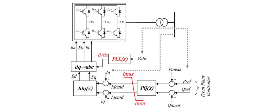
Figure 1 - Block diagram of a GFL inverter
GFM inverters, as the name suggests, can generate their own voltage and frequency references, and do not need to detect the grid voltage phase angle and frequency for stable operation. However, these devices will still need to maintain synchronism with the connected grid to operate stably. The high-level block diagram of a GFM inverter is shown in Fig. 2. In this control method, the PQ(s) control block generates the internal voltage, angle and frequency signal based on the active and reactive power requirements. The Eθ(s) block then generates the d and q-axis current commands that are used by the current controller Idq(s) to appropriately control the switching of the IGBTs. It is important to mention that for GFM technologies the internal voltage, angle and frequency can be created using multiple control paradigms like droop control, virtual synchronous machine, dispatchable voltage-controlled oscillator to name a few [3], [4]. In addition to that, GFM inverters may also have a single loop controller, where instead of having a current (Idq(s)) controller, the internal voltage can be controlled directly [20]. A detailed discussion and comparison of these different control methods is beyond the scope of this work and will not be pursued here. Instead, this work will focus on the general ability of IBRs either GFM or GFL to operate stably and provide grid support following faults on the grid. It is also worthwhile to point out that both GFM and GFL technologies are voltage source inverters that can be either current controlled or voltage controlled [21].
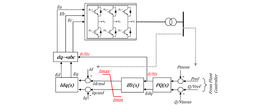
Figure 2 - Block diagram of a GFM inverter
3. Inverter performance following a fault
IBRs perform significantly differently as compared to SM during grid fault conditions. Among other things, the overloading capability of IBRs is significantly different from a SM. During faulted conditions, when the terminal voltage is depressed, SMs can supply routinely 3.5 to 4 pu current transiently (before the over excitation limiter steps in) [22]. This stator overloading capability helps SMs to supply the reactive power support that helps with voltage recovery. IBRs on the other hand can be restricted in its overloading capability due to the limitations associated with the IGBTs. To avoid damaging the IGBTs, IBRs employ fast current limiters that can limit the current within the inverter’s allowable limits. Unless oversized, the IBRs are generally rated to handle 1.2 to 1.5 pu (per unit on the plant’s MVA base) current [23]. It has been reported that some GFM inverters, particularly the ones that utilize energy storage, can inject between 2 to 3 pu current (per unit on the plants MVA base) during fault conditions [24]. The limited current injection capability of IBRs (both GFL and GFM) can exacerbate the voltage recovery after a fault, especially in regions with large numbers of small inertia single and three phase induction motors which are known to cause delayed voltage recovery [18]. In addition, multiple studies have also indicated that GFM inverters can be prone to instability when operating at the current limit [8], [9], [25]. It is therefore important to understand the operation of GFL and GFM inverters specially during these delayed voltage recovery conditions as these resources replace the existing fleet of SMs.
Fig. 3 shows the phasor diagram of a GFL IBR’s voltage and current during normal and current limited with depressed voltage operating conditions. Einv is the internal inverter voltage, Vt is the terminal voltage, θ is the phase angle of the phasor Vt, Iinv is the inverter current and Idinv and Iqinv are the d-axis and q-axis components of Iinv . The relationships between these phasor quantities are given by:
(1)
(2)
(3)
(4)
(5)
where, quantities with subscripts d and q are the d and q axis components, and R and X are the impedances between the terminal of the IBR to the internal voltage. These are typically the IBR filter impedances. For current controlled voltage source inverters, the Idcmd and Iqcmd current references are generated by the current controller PQ(s) (for GFL see Fig. 1) or Eθ(s) (for GFM see Fig. 2). These are in turn used to generate the values of Ed and Eq using equations (1) and (2) in steady state, which determines Einv and its phase angle. These equations apply to both GFL and GFM inverters that are current controlled [3], [4].
During normal operation, θ is tracked by the PLL and current is injected with a phase lead or lag depending upon the active and reactive power set points. During depressed voltage conditions (reduced Einv and Vt) when the IBR is at its current limit, depending on the active (P) or reactive (Q) power priority, the magnitudes of d-axis and q-axis currents are calculated [19]. This determines the phase lag between Vt and Iinv and in turn the P and Q output in that condition. The extreme case when the inverter is operating on Q priority with Iq being at Imax is shown in Fig. 3. The inverter tries to maximize the Q output in this condition at the expense of P. The current limit, Imax, determines the voltage support capability of the GFL, whereas the ability of the GFL to track the phase of Vt will determine its ability to operate stably. It is well known that GFL inverters can run into challenges while tracking the phase when connected to a weak grid [7].
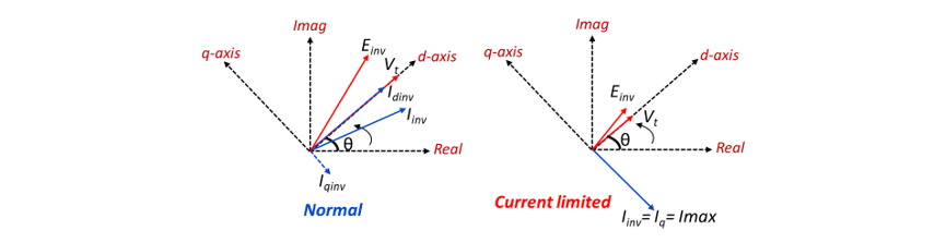
Figure 3 - Qualitative phasor diagram of GFL quantities under normal and current limited with depressed voltage operation
Fig. 4 shows the qualitative phasor diagram of the GFM quantities under normal and current limited with depressed voltage operation. Under normal operation, the internal voltage magnitude Einv and the angle θ is controlled (Einv is aligned with the d-axis) to achieve the desired active and reactive power output. When the inverter is at its current limit, the values of Id and Iq are fixed by the current limiter logic. Inspecting (1) and (2), one can see that with fixed values of Id and Iq the inverter can no longer control Ed and Eq (or Einv and its phase θ (see (3)) to a desired value. Instead, it injects fixed values of q-axis and d-axis currents with the d axis angle θ controlled by Eθ(s), effectively injecting Iinv at an angle θ instead of controlling Einv at an angle θ. This is unlike the normal operating condition, where Einv is held at an angle θ. Furthermore, since Iinv is injected at an angle θ with an arbitrary reference (and not Vt see Fig. 4), The active and reactive power output of the GFM inverter cannot be controlled precisely during this condition, unless additional controls exist to track the phase angle of Vt in a GFM inverter.
Additionally, irrespective of the type of control method, GFMs have an active power-frequency and reactive power-voltage relationship, which in the steady state is given by [26]:
(6)
(7)
where, ω is the frequency, Vt is the terminal voltage, Pref and Pmeas are the reference and measured active power respectively, Qref and Qmeas are the reference and measured reactive power respectively, and Kpf and Kqf are the active and reactive power droops respectively. This relationship is maintained so that GFM inverters can emulate the droop response of SMs in an interconnected system. These concepts are explained in [26]. Hence, when the active power output of GFM drops under depressed terminal voltage condition, the angle θ of inverter can accelerate and cause the current injection to become out of phase with the terminal voltage resulting in a phenomenon like a SM’s rotor angle accelerating beyond 180 degrees. This presents a stability challenge for a GFM inverter under depressed voltage condition [8], [9], [25]. Note that since the angle θ phenomenon is dependent on the dynamics given by (6) which is common to all GFM technologies, this type of stability risk can be a challenge for GFMs of all control philosophies.
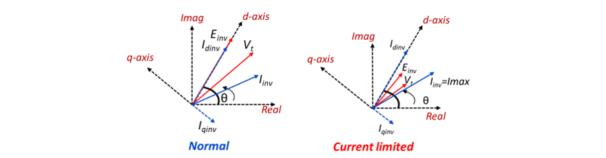
Figure 4 - Qualitative phasor diagram of GFM quantities under normal and current limited operation
Based on the description provided here, it is important to assess the operability of IBRs, both GFL and GFM under conditions that can result in slow voltage recovery, as such conditions can often be accompanied by IBRs operating at or near their current limits for extended periods of time (unless IBRs are significantly oversized). Since the voltage recovery of the system is strongly dependent on the local load, the performance of GFM as well as GFL inverters need to be studied when serving different type of local load. The next section describes the test system, the models and the different load conditions studied to evaluate performance of IBRs following a fault.
4. Test system description
The test system used for this study is shown in Fig. 5. The test system has 158 MW of local load (a combination of 120 MW of dynamic and 38 MW of static load) and 134 MW of local generation. The study system is connected to an external grid dominated by SMs via two transmission paths. One of these transmission paths is assumed to be an electrically shorter connection to the external grid with a lower impedance, while the other path is electrically longer and has a higher impedance. The fault event simulated for this study is a 3-phase line to ground fault on the shorter transmission paths followed by disconnection of the line to clear the fault in 5 cycles. Two separate post-fault grid topologies were investigated. In the first case, it is assumed that after the removal of the faulted line the short circuit ratio (SCR) at bus 1000 is 3.7 [1]. In the second case, the impedance of the remaining path is increased to bring down the SCR at bus 1000 to 1.5. These two cases were created to study the effect of grid weaking.
To assess the concerns with GFL and GFM technologies a set of studies were conducted with the local load and generation being represented by different generator technologies and load types. The system response for each combination of load and generation type listed in Table 1 were evaluated in this study.
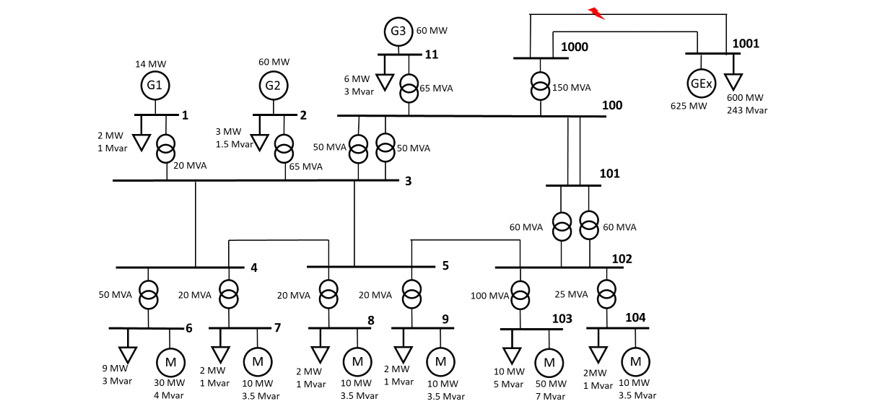
Figure 5 - Test system used for the study
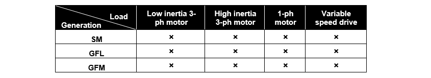
Table 1 - Generation types and types evaluated to study system performance
To simulate the system dynamics, the synchronous machines were represented with a 5-state round rotor generator model [27]. The generator is equipped with a ST1 excitation system model [28], with separate over and under excitation limiters. The governors on the synchronous machines are modeled using a general-purpose GE gas turbine model, GGOV1 [29]. These models are available in all leading power system simulators. A round rotor generator model with a static excitation system and a gas turbine represents one of the most common configurations of a conventional synchronous generator. For modeling the GFL inverters the second-generation renewable generator models (the repc, reec, and regc, model family) developed by the Western Electricity Coordinating Council’s (WECC’s) Renewable Energy Modeling Task Force were used [30]. For the GFM inverters, the model first introduced in [31] was used. Both GFM and GFL inverters models use parameter values that are within ranges based on engineering experience. This type of parameterization is suitable for the exploratory study presented here that highlights the risks. For actual site-specific studies, it is strongly recommended that these models are parameterized via validation studies in consultation with actual equipment manufacturer [32]. The complete set of parameters for the generator models used in this paper are provided in the Appendix.
For the load models, the low and high inertia 3-phase motor loads are represented using the 5-state induction motor models [33]. Low inertia 3-phase motor loads have inertia constants in the range 0.1-0.4 s. Low inertia motor loads typically represent pumps and positive displacement compressor type loads which have comparatively smaller dimensions. High inertia 3-phase motor loads have inertia constants in the 0.6-1s range [33]. High inertia motor loads typically represent different types of fans and centrifugal compressors which have larger dimensions as compared to the low inertia motor loads. Note that other types of motor loads fall in these low and high inertia categories, but fans, pumps and compressors are most common continuous duty loads in the power system. 1-phase motors are represented using a phasor representation explained in [34]. 1-phase motors have even smaller inertia constants that ranges between 0.01-0.04s [34]. These are typically found in residential applications. The variable speed drives (VSD) are represented by the aggregated VSD model developed in [35]. Detailed parameters of the load models are listed in the Appendix. It is important to mention that for dynamic assessment in this study the loads are represented as an aggregation of several loads connected at that bus. As an example, the 50 MW load at bus 103 is not a single large 50 MW load, but a collection of smaller loads with individual consumptions summing up to 50 MW. Further details on aggregated load modeling can be found in [36]. The loads are assumed to have power factors ranging between 0.9 to unity. This is a fair assumption as most load sites have power factor correction mechanisms to ensure proper steady state power factor. It is important to mention that although important, the steady state power factor of the load is not a key contributing factor in the phenomena described later in the paper. Rather, the transient reactive power consumption of the loads during disturbances has a critical impact on the stability of the local devices. In general, if the load power factor is poor and power factor correction devices are not employed, it predisposes the system to both voltage and transient stability issues and increases the chances of the occurrence of the issues described later in the paper.
A commercial positive sequence phasor-based power system simulator was used to perform the study for this work. The stability issues that are highlighted in forthcoming sections are for balanced faults and in the frequency range that can be handled by positive sequence simulators with sufficient fidelity. Hence, such a simulator was chosen. These results can also be replicated using an electromagnetic transient (EMT) simulator. This however does not indicate that all issues with IBRs can be studied in a positive sequence framework and EMT simulators are preferred for a whole range of studies, a discussion of which is beyond the scope of this paper. Furthermore, it is worthwhile to emphasize that IBR technology is evolving, and issues noted here should not be considered as absolute. Rather the findings of this study are meant to highlight the issues that engineers should be mindful of while evaluating the benefits of different technologies.
5. Fault Response with a post fault SCR of 3.7
As indicated before, the system response was studied for different combinations of local load and generation. For the initial assessment, to emphasize on the impact of current limitation, the GFM and GFL are both assumed to have a maximum current limit of 1.2 pu. The current limited is implemented via a circular limiter for the d-q axis such that
(8)
For the initial set of results for both GFM and GFL inverters, it is assumed that under current limits, the Iq will be maximized at the expense of Id. This is also called Q-priority for GFL inverters. For GFM inverters, the relevance of this prioritization is still a research topic, but such an investigation is beyond the scope of this work.
Local load modeled as high-inertia 3-phase motors
Fig. 6 shows the system response with the loads modeled as high-inertia 3-phase motors. The three sets of curves in each plot shows the responses when all the local generators are modeled as SMs, GFL inverters and GFM inverters respectively. From the responses shown here, the system can operate stably without any issues irrespective of whether the local generation is SMs or IBRs using GFL or GFM technology. It is also interesting to note that the SMs have a notably oscillatory response (at approx. 1 Hz) compared to the IBRs. The same can be noted for all the simulation results presented in this paper. These oscillations are due to the electro-mechanical modes in SMs that are absent in IBRs. Additionally, a voltage spike is observed in the case of the GFL IBR. This spike is due to the control settings of models used and can be adjusted for a more suitable response. Since the issue investigated here was the stable operation of IBRs, such adjustments were neglected for this work. Furthermore, the fluctuations in the MW and Mvar output of the GFL IBR is due to its Q-priority operation that curtails MW to produce Mvar for supporting voltage. Additionally, in Fig. 6 (d) it can be seen that the on-fault voltage with SMs are generally higher than that with GFL or GFM IBRs. This is due to the higher short-circuit contribution from SMs during the fault. This trend is common for all the simulations performed in this paper and hence for brevity detailed on-fault voltages will not be shown as a sub plot for the remaining figures in the paper.
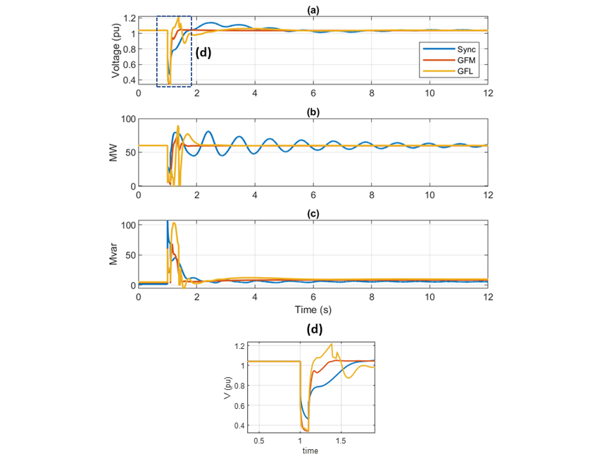
Figure 6 - (a) Terminal voltage, (b) MW output, (c) Mvar output, (d) detailed on-fault voltage of the generator connected at Bus 11 with local loads modeled as high inertia 3-phase motors

Local load modeled as low-inertia 3-phase motors
Fig. 7 shows the system response with loads modeled as low-inertia 3-phase motors. The voltage recovery in this case is slower than that observed in Fig. 6. This is due to the high reactive power consumption of small motors caused by rapid deceleration followed by acceleration of these motors after the fault. From the responses shown here, the system can operate stably (with a slower voltage recovery) when the generators are either SMs or GFL inverters. SMs, due to their higher stator loading capability can support the system voltage, provide active power, and maintain stability. The GFL IBRs, due to their Q-priority mode, maximize the Mvar output by curtailing the MW. The GFL inverters in this case can operate stably as the PLL continues to track the system voltage after the fault is cleared. However, when GFM inverters are used for the local generators, the system goes unstable, with voltage oscillations indicative of loss of synchronism. The instability seen in the case of GFM IBRs is due to the inverters hitting their current limit under depressed voltage. This phenomenon is described in the previous section.
In addition to the instability noted for the GFM IBRs in Fig. 7, the depressed voltages for the GFL IBRs and SMs can be seen to rise sharply around 3s. The sharp voltage recovery seen here is due to the quick reacceleration of the low inertia 3-phase motors in the system, which causes their reactive power consumption to drop sharply. Fig. 8 (a) shows the per unit rotor speeds and Fig. 8 (b) shows the Mvar consumption of the motors connected to bus 103 for the case with GFL IBR and SMs.
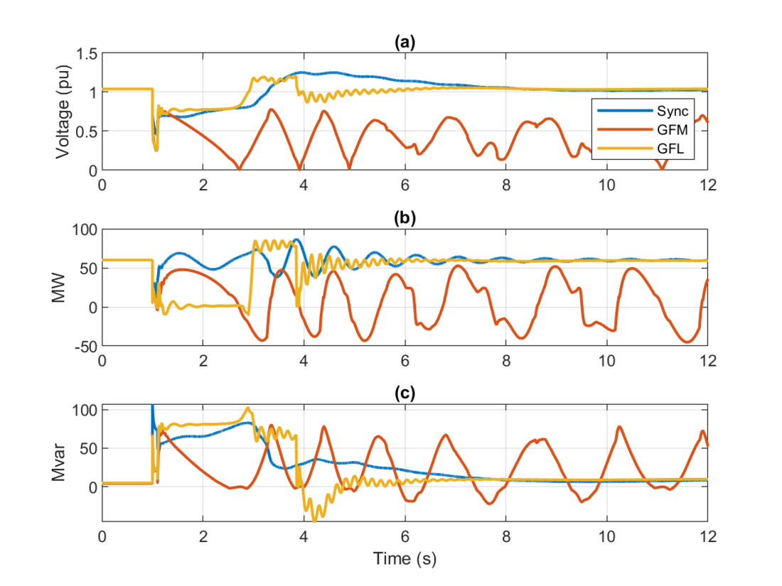
Figure 7 - (a) Terminal voltage, (b) MW output and, (c) Mvar output of generator connected at Bus 11 with local loads modeled as low inertia 3-phase motors
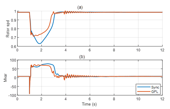
Figure 8 - (a) Rotor speed, (b) Mvar consumption of low inertia 3-phase motors connected at bus 103
Local load modeled as 1-phase motors
Fig. 9 shows the system response with loads modeled as 1-phase motors driving a compressor type load. From the responses shown here, the system can operate stably when the generators are SMs or GFL inverters, although the voltage recovery is notably slower than that observed in Fig. 6 and Fig. 7. The operation of the GFL IBRs and SMs in this case is similar to the case with low-inertia 3 phase motors. The slow voltage recovery observed here is due to the complete stalling of the 1-phase motors followed by their tripping on thermal protection. The tripping of 1-phase motors results in reduced system load that causes the system voltage to exceed the pre-disturbance level as seen for the case with SMs (blue curve). These type of local overvoltages due to tripping of 1-phase motors after fault has been reported in various literature [15], [16]. Furthermore, like the case with small inertia 3 phase motors, when GFM inverters are used for the local generators, the system goes unstable, with voltage oscillations indicative of loss of synchronism. The instability with GFM IBRs seen in this case is also due to the inverters hitting their current limit under depressed voltage.
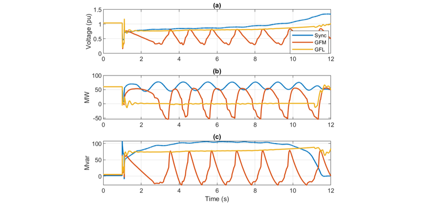
Figure 9 - (a) Terminal voltage, (b) MW output and, (c) Mvar output of generator connected at Bus 11 with local loads modeled as 1-phase motors
Local load modeled as VSD
Fig. 10 shows the response of the system with the local loads modeled as VSDs. From the responses shown here, the system can operate stably without any issues irrespective of whether the local generation is SMs or IBRs using GFL or GFM technology. Furthermore, no slow voltage recovery is observed in this case.
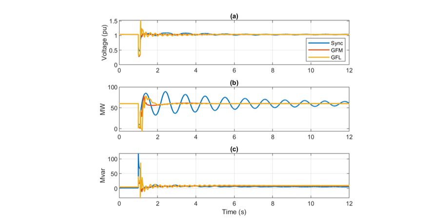
Figure 10 - (a) Terminal voltage, (b) MW output and, (c) Mvar output of generator connected at Bus 11 with local loads modeled as VSDs
Analysis of results
The simulations presented here indicate that the system is stable irrespective of whether the local generators are SMs or IBRs (GFL and GFM) when the local loads do not hinder voltage recovery and the external tie is strong. This is typically true when the load comprises of large inertia motors or VSDs. If the local loads cause slow voltage recovery (as in the case with low inertia 3-phase motors and 1-phase motors) the effect of the 1.2 pu current limit on GFL and GFM inverters is far more evident. When GFL inverters are used, the system is stable, however, the voltage recovery becomes poorer as compared to SMs in the case when the local loads are 1-phase motors. The system performance is even worse when GFM inverters are used as these lose synchronism when operating under current limit for an extended duration, driven by the slow voltage recovery. Fig. 11 shows the phase angle between the terminal voltage (Vt) and inverter current (Iinv) of the GFM IBR at Bus 11, for the case where the local loads are 1-phase motors. As explained in the previous section, the depressed terminal voltage causes the phase angle between Vt and Iinv to increase leading to a loss of synchronism, which is indicated by the phase angle between Vt and Iinv going past 90 degrees resulting in reverse active power at the 2.95s mark.
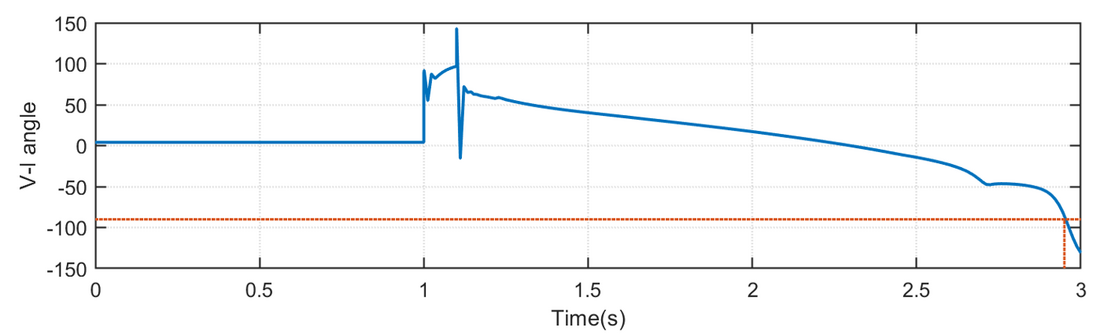
Figure 11 - Angle between terminal voltage and current of the GFM inverter at Bus 11
To emphasize that this effect of current limits, the simulations using GFL and GFM inverters were repeated by setting Imax to 1.9 pu (see Fig. 12) for the two critical scenarios where the local loads are 3-phase small inertia motors and 1-phase motors. With the increased current limit, the system responses are significantly better as compared to those in Fig. 7 and Fig. 9 . Notably, the GFM inverters continue to operate stably when the current limit is increased. Additionally, the voltage recovery looks better with both GFM inverters and GFL inverters compared to the SMs as the inverters can now inject more reactive power to support the voltage. Note that the repeated voltage dips observed in Fig. 12 (b) for the GFL inverter case (yellow trace) after 9 s are caused by high voltage current blocking feature in GFL inverters which blocks the current as the terminal voltage reaches 1.2 pu [30]. The current block causes the inverter to cease operation momentarily causing the voltage to dip. It is worthwhile to mention that the trend of the voltage recovery is the focus here rather than the shape of the actual curves. The shape of this recovery needs to be ascertained for specific sites using validated parameter sets.
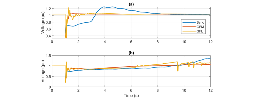
Figure 12 - Terminal voltage of generator at Bus 11 for an Imax of 1.9 pu for the IBRs when local loads are (a) small inertia 3-phase motors and, (b) 1-phase motors
6. Fault Response with a Post Fault SCR of 1.5
In this section, it is assumed that the remaining tie is a weaker link. Under this condition the simulations are repeated assuming the local loads are (a) 1-phase motors, (b) low inertia 3-phase motors, and (c) high inertia 3-phase motors. The current limit was set to 1.9 pu for the IBRs for this set of runs as it was already established in the previous simulations that the lower current limit causes the GFM inverters to become unstable. The parameters of the SM were left unchanged. Fig. 13 shows the responses of the system following the fault.
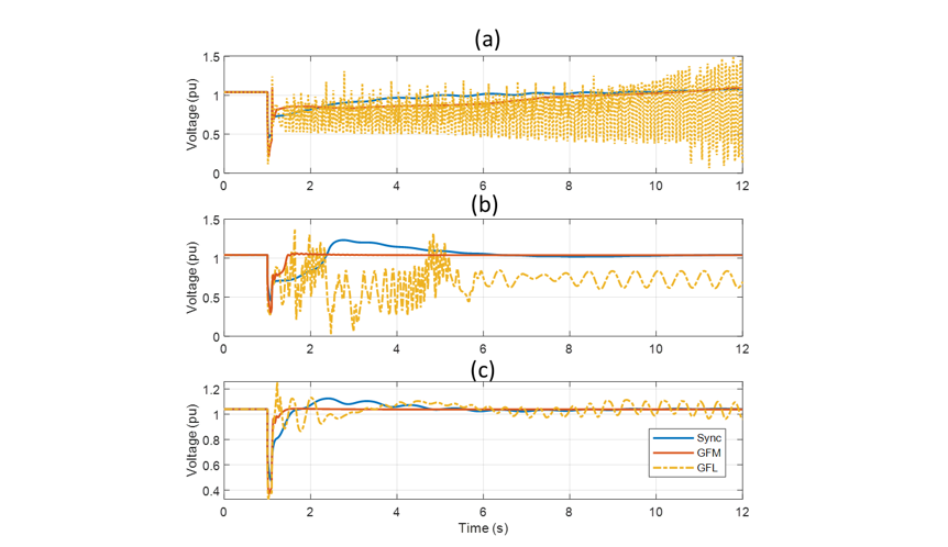
Figure 13 - Terminal voltage of IBRs at Bus 11 with a weak external tie when local loads are (a) 1-phase motors (b) 3-phase low inertia motors, and (c) 3-phase high inertia motors
It can be seen that properly sized GFM inverters and SMs are clearly a more suitable option for regions which might have weak connections to the external grid. Furthermore, irrespective of the type of local load, oscillatory issues were observed with the GFL IBRs. The performance issues of GFL inverters in weak grids and the benefits of GFM inverters under these conditions are well known and have been documented in various studies [7].
7. Conclusions
The results presented in this work highlight some of the concerns with stable operation of IBRs during grid events like faults that can result in slow voltage recovery or cause weakening of the grid at the point of concern. Some of the key takeaways from the study are as follows:
- When IBRs are in portions of the system where the local load is not expected to cause delayed or slow voltage recovery, and the fault clearance does not render the local system weak, both GFM and GFL technologies can perform well without any issues related to stability or loss of synchronism.
- If the local load is predominantly small motors (both 3-phase and 1-phase) that can cause slow voltage recovery, GFM inverters can run into stability issues if the low voltage condition causes the device to operate at its current limit for extended periods of time without being able to push active power. GFL inverters in this situation can still operate stably if the PLL can track the system frequency properly. However, the current limits on GFL limits its ability to supply reactive power support that can result in poorer voltage recovery as compared to the case if the generators were SMs.
- Increasing the current limits on GFM inverters by oversizing the inverters, helps the GFM inverters to operate stably as well as improve the voltage recovery in that area. Increasing current limits on GFL inverters do not enhance the stability of the devices when connected to a weak system, however it does help with better voltage recovery which might be necessary in some regions to prevent cascaded trip of other resources.
- When a grid fault and subsequent fault clearing results in weakening of the local system, GFM inverters with appropriate current limits have an advantage over GFL inverters which may have issues operating stably due to the hierarchy of their control structure.
It is important to mention that the results presented here highlight the concerns that transmission planners and operators should be mindful of while evaluating the performance of IBRs for their system. Additionally, oversizing inverters may not be the only solution to the issues mentioned here. IBRs, both GFM and GFLs, are highly controllable devices and control-based solutions may be possible to achieve stability under different operating conditions. Utilities should consult IBR manufacturers to identify such solutions. Other solutions may include adding local dynamic voltage support using static compensators (STATCOMs) or synchronous condensers. A detailed study, using proper local load models as well as manufacturer verified IBR models should be used to evaluate these mitigation measures. The main contribution of this work was to highlight the challenges associated with maintaining IBR stability during slow voltage recovery conditions. The work also highlights the importance of load modeling. Without the use of proper and reasonable load models, the issues reported in this work cannot be replicated or studied. The investigation of mitigation measures to ensure IBR stability is still work in progress and is expected to be a subject of future work. Furthermore, studies assessing the system response with different proportions of SMs and IBRs in the local system and the associated stability concerns will be subject of future work.
References
- Denis, G., Prevost, T., Panciatici, P., et al: ‘Review on potential strategies for transmission grid operations based on power electronics interfaced voltage sources,’ 2015 IEEE Power Energy Society General Meeting, 2015, pp. 1–5
- J. Matevosyan, et al., “Grid-Forming Inverters: Are They the Key for High Renewable Penetration?” IEEE Power and Energy Magazine, vol. 17, no. 6, pp 89-98, Oct. 2019.
- High Share of Inverter-Based Generation Task Force. 2022, Grid-Forming Technology in Energy Systems Integration. Reston, VA: Energy Systems Integration Group. https:// www.esig.energy/reports-briefs
- Lin, Yashen, Joseph H. Eto, Brian B. Johnson, Jack D. Flicker, Robert H. Lasseter, Hugo N. Villegas Pico, Gab-Su Seo, Brian J. Pierre, and Abraham Ellis. 2020. Research Roadmap on Grid-Forming Inverters. Golden, CO: National Renewable Energy Laboratory. NREL/TP-5D00-73476. https://www.nrel.gov/docs/fy21osti/73476.pdf.
- Grid Forming Inverters: EPRI Tutorial. EPRI, Palo Alto, CA: 2022. 3002025483
- Rick Wallace Kenyon, et al., “Stability and control of power systems with high penetrations of inverter-based resources: An accessible review of current knowledge and open questions,” Solar Energy, https://doi.org/10.1016/j.solener.2020.05.053
- W. Wang, et al., “Instability of PLL-synchronized converter-based generators in low short-circuit systems and the limitations of positive sequence modeling,” Proc. of the IEEE North American Power System, 2018, USA
- M.G. Taul, X. Wang, P. Davari, F. Blaabjerg, “Current Limiting Control with Enhanced Dynamics of Grid-Forming Converters during Fault Conditions,” IEEE Journal of Emerging and Selected Topics in Power Electronics, vol. 8, no. 2, pp 1062-1073, July 2019.
- T Qoria, et. al.,” Current limiting algorithms and transient stability analysis of grid forming VSCs,” Electrical Power System Research, vol. 189, Dec. 2020.
- Wang, Jing, and Govind Saraswat. 2022. Study of Inverter Control Strategies on the Stability of Low-Inertia Microgrid Systems: Preprint. Golden, CO: National Renewable Energy Laboratory.
- F.P. deMello, J.W. Feltes, “Voltage oscillatory instability caused by induction motor loads,” IEEE Trans. on Power Syst., vol. 11, no. 3., pp1279-1285., Aug 1996.
- J. V. Milanovic and I. A. Hiskens, “Effects of load dynamics on power system damping,” IEEE Trans. Power Syst., vol. 10, no. 2, pp. 1022–1028, May 1995.
- D. N. Kosterev, C. W. Taylor, W. Mittlestadt, “Model Validation for the August 10,1996 WSCC System Outage,” vol 14, no 3, pp. 967 – 979, Aug. 1999.
- P. Mitra, D. Ramasubramanian, A. Gaikwad, “Impact of Load Modeling on Power System Oscillations,” Proc IEEE PES General Meeting 2022, Denver CO.
- Williams, B.R., W.R. Schmus, and D.C. Dawson. "Transmission voltage recovery delayed by stalled air conditioner compressors." IEEE Transactions on Power Systems, vol 7, no. 3, pp 1173-1181, 1992.
- Shaffer, J.W. "Air conditioner response to transmission faults." IEEE Transactions on Power Systems, vol. 12, no. 2, pp 614-621, 1997.
- Taylor, L.Y., and Shih-Min Hsu. "Transmission voltage recovery following a fault event in the Metro Atlanta area." IEEE PES Summer Meeting, 2000.
- L. Sundaresh, et. al., “Impact of large-scale integration of inverter-based resources on FIDVR,” Proc. IEEE North American Power Symposium, AZ, USA, 2020.
- Program on Technology Innovation: Benefit of Fast Reactive Power Response from Inverters in Supporting Stability of Weak Distribution Systems: A Use Case of Grid Forming Inverters and the Performance Requirements, EPRI Palo Alto, CA: 2020, 3002020197
- W. Du, et. al., “A Comparative Study of Two Widely Used Grid-Forming Droop Controls on Microgrid Small Signal Stability,” IEEE Journal of Emerging and Selected Topics in Power Systems, vol. 8, no. 2, pp 963-975, Sept. 2019.
- E. Muljadi, M. Singh, and V. Gevorgian, NREL Report: User Guide for PV Dynamic Model Simulation Written on PSCAD Platform, NREL/TP-5D00-62053, Nov 2014, available online: https://www.nrel.gov/docs/fy15osti/62053.pdf
- IEEE C50.13-2014 - IEEE Standard for Cylindrical-Rotor 50 Hz and 60 Hz Synchronous Generators Rated 10 MVA and Above. https://standards.ieee.org/standard/C50_13-2014.html
- G. Kou, et. al., “Fault Characteristics of Distributed Solar Generation,” IEEE Trans. on Power Delivery, vol. 35, no. 2, pp 1062-1064, Apr 2020.
- N. S. Gurule, et. al., “Grid-forming Inverter Experimental Testing of Fault Current Contributions,” Proc. IEEE 46th Photovoltaic Specialists Conference (PVSC), June 2019, IL, USA.
- C. Schöll, H. Lens, "Impact of Current Limitation of Grid-forming Voltage Source Converters on Power System Stability", IFAC-Papers Online, Vol. 53, Issue 2, 2020, Pages 13520-13524.
- B. Johnson, et. al, “A Generic Primary-control Model for Grid-forming Inverters: Towards Interoperable Operation & Control,” Proceedings of the 55th Hawaii International Conference on System Sciences, 2022.
- 1110-2019 - IEEE Guide for Synchronous Generator Modeling Practices and Parameter Verification with Applications in Power System Stability Analyses.
- 421.5-2016 - IEEE Recommended Practice for Excitation System Models for Power System Stability Studies
- Dynamic Models for Turbine-Governors in Power System Studies, PES TR1 Technical Report, Prepared by: IEEE Power System Stability Subcommittee, Task Force on Turbine-Governor Modeling, 2013.
- WECC Report: Solar Photovoltaic Power Plant Modeling and Validation Guideline, prepared by WECC Model Validation Working Group, 2019.
- Generic Positive Sequence Domain Model of Grid Forming Inverter Based Resource, EPRI Palo Alto, CA: 2021, 3002021403
- P. Pourbeik, N. Etzel, S. Wang, “Model Validation of Large Wind Power Plants Through Field Testing,” IEEE Trans. Sustainable Energy, vol. 9, no. 3, pp. 1212-1219, 2017.
- P. Kundur, Power system stability and control. New York, NY, USA: McGraw-Hill, 1994.
- B. Lesieutre, D. Kosterev, J. Undrill, “Phasor modeling approach for single phase A/C motors,” in Proc. 2008 IEEE PES GM, Pittsburgh, PA, USA, July 2008
- P. Mitra, D. Ramasubramanian, A. Gaikwad, J. Johns, “Modeling the aggregated response of variable frequency drives (VFDs) for power system dynamic studies,” IEEE Trans. on Power Syst. vol. 35, no. 4, pp2631-2641, 2020
- Technical Guide on Composite Load Modeling: EPRI, Palo Alto, CA: 2017. 3002019209.
Appendix
Generator Model Parameters (model name gentpj)
"tpdo" 6.0000 "tppdo" 0.0250 "tpqo" 0.8000 "tppqo" 0.0500 "h" 5.0000 "d" 0.0000 "ld" 2.2000 “lq" 2.1000 "lpd" 0.2000 "lpq" 0.6400 "lppd" 0.1800 "lppq" 0.1800 "ll" 0.1500 "s1" 0.0800 "s12" 0.5000 "ra" 0.0000 "rcomp" 0.0000 "xcomp" 0.0000 "accel" 0.4000 "kis" 0.0000
Excitation System Model Parameters (model name exst1 (ST1A))
"tr" 0.0 "vimax" 1.000000 "vimin" -1.000000 "tc" 1.000000 "tb” 10.0000 "ka" 200.00 "ta" 0.050000 "vrmax" 5.0000 "vrmin” -5.0000 "kc" 0.0 "kf" 0.0 "tf" 1.000000 "tc1" 0.0 "tb1" 0.0 "vamax” 99.0000 "vamin" -99.0000 "xe" 0.0 "ilr” 99.0000 "klr" 0.0
Overexcitation limiter model (model name oel1)
"ifdset" 2.5000 "ifdmax" 3.5000 "tpickup" -10.0000 "runback" 0.0 "tmax" 60.0000 "tset" 60.0000 "ifcont" 3.0000 "vfdflag" 0.0 "alarm" 0.0
Governor model (model name ggov1)
"r" 0.050000 "rselect" 1.000000 "tpelec" 1.000000 "maxerr" 1.000000 "minerr" -0.100000 "kpgov" 10.0000 "kigov" 1.000000 "kdgov" 0.0 "tdgov" 1.000000 "vmax" 1.000000 "vmin" 0.150000 "tact" 0.500000 "kturb" 1.5000 "wfnl" 0.180000 "tb" 0.200000 "tc" 0.0 "flag" 1.000000 "teng" 0.0 "tfload" 3.0000 "kpload" 3.0000 "kiload" 1.000000 "ldref" 1.000000 "dm" -2.0000 "ropen" 3.3000 "rclose" -3.3000 "kimw" 0.0 "pmwset" 18.0000 "aset" 0.010000 "ka" 10.0000 "ta" 0.200000 "db" 0.0 "tsa" 4.0000 "tsb" 5.0000 "rup" 99.0000 "rdown" -99.0000 "tbd" 0.0 "tcd" 0.0 "ffa" 0.0 "ffb" 0.0 "ffc" 0.0 "dnrate" 0.000200 "dnhi" 0.100000 "dnlo" -0.100000 "t1" 0.0 "t2" 0.0 "t3" 0.0 "t4" 0.0 "t5" 0.0 "n1" 0.0 "n2" 0.0 "n3" 0.0 "n4" 0.0 "n5" 0.0
GFL IBR generator model (model name regc_c)
"tfltr" 0.020000 "te" 0.010000 "rrpwr” 10.0000 "re" 0.002000 "xe" 0.200000 "iqrmax" 999.00 "iqrmin" -999.00 "rateflg" 0.0 "imax" 1.9000 "dqflag" 0.0 "kip" 2.0000 "kii" 40.0000 "kppll" 20.0000 "kipll" 1200.00 "wmax" 75.4000 "wmin" -75.4000 "vdip" 0.600000
GFL IBR electrical controller model (model name reec_d)
"vdip" 0.500000 "vup" 1.1000 "trv" 0.020000 "dbd1" -0.050000 "dbd2" 0.050000 "kqv" 2.0000 "iqh1" 1.0500 "iql1" -1.0500 "vref0" 1.000000 "iqfrz" 0.0 "thld" 0.0 "thld2" 0.0 "tp" 0.050000 "qvmax" 99.0000 "qvmin" -0.436000 "vmax" 1.1000 "vmin" 0.900000 "kqp" 0.0 "kqi" 0.500000 "kvp" 0.0 "kvi" 40.0000 "vref1" 0.0 "tiq" 0.020000 "dpmax" 99.0000 "dpmin" -99.0000 "pmax" 1.1200 "pmin" 0.040000 "imax" 1.9000 "tpord" 0.020000 "vcmpflag" 1.000000 "pfflag" 0.0 "vflag" 1.000000 "qflag" 1.000000 "pflag" 0.0 "pqflag" 0.0 "rc" 0.0 "xc" 0.0 "tr1" 0.030000 "kc" 0.0 "ke" 0.0 "vblkh" 1.2000 "vblkl" 0.100000 "tblkdelay" 0.050000 "vq1" 0.0 "iq1" 1.9000 "vq2" 0.100000 "iq2" 1.9000 "vq3" 0.200000 "iq3" 1.9000 "vq4" 0.500000 "iq4" 1.9000 "vq5" 1.000000 "iq5" 1.9000 "vq6" 1.2000 "iq6" 1.9000 "vq7" 2.0000 "iq7" 1.9000 "vq8" 0.0 "iq8" 0.0 "vq9" 0.0 "iq9" 0.0 "vq10" 0.0 "iq10" 0.0 "vp1" 0.0 "ip1" 1.9000 "vp2" 2.0000 "ip2" 1.9000 "vp3" 0.0 "ip3" 0.0 "vp4" 0.0 "ip4" 0.0 "vp5" 0.0 "ip5" 0.0 "vp6" 0.0 "ip6" 0.0 "vp7" 0.0 "ip7" 0.0 "vp8" 0.0 "ip8" 0.0 "vp9" 0.0 "ip9" 0.0 "vp10" 0.0 "ip10" 0.0
GFL IBR plant control model (model name repc_a)
"tfltr" 0.020000 "kp" 1.000000 "ki" 3.0000 "tft" -0.050000 "tfv" 0.050000 "refflg" 1.000000 "vfrz" 0.850000 "rc" 0.0 "xc" 0.0 "kc" 0.0 "vcmpflg" 0.0 "emax" 99.0000 "emin" -1.000000 "dbd" 0.0 "qmax" 99.0000 "qmin" -99.0000 "kpg" 1.000000 "kig" 2.0000 "tp" 0.250000 "fdbd1" 0.0 "fdbd2" 0.0 "femax" 999.00 "femin" -999.00 "pmax" 1.000000 "pmin" 0.0 "tlag" 0.100000 "ddn" 20.0000 "dup" 0.0 "frqflg" 1.000000 "outflag" 0.0 "puflag" 1.000000
GFM IBR full model (refer to [31] for model description)
"rsrc" 0.0015 "xsrc" 0.1500 "Cf" 0.0167 Vdip" 0.0000 "Imax" 1.2000 "pqflag" 1.0000 "control" 1.0000 "m_f" 0.1500 d_f" 30.0000 "Tr" 0.0030 d_d" 0.0000 "d_v" 22.2200 "Kppll" 20.0000 "Kipll" 200.0000 "K_Pv" 2.5000 "K_Iv" 10.0000 "K_Pi" 0.1000 "K_Ii" 5.0000 "Te" 0.0050 "K_Pp" 0.5000 "K_Ip" 20.0000 "K_Pvq" 0.5000 "K_Ivq" 150.0000 "Kpvq" 0.0000 "Kivq" 0.0000 "K_pod" 0.0000 "Tw_pod" 0.0100 "T1_pod" 0.0100 "T2_pod" 0.0050 "Pmax" 1.0000 "Pmin" 0.0000 "Qmax" 1.0000 "Qmin" -1.0000 "Kp_plim" 1.0000 "Ki_plim" 0.1000 "Kp_qlim" 0.1000 "Ki_qlim" 1.5000 "Tfrz" 0.2000
High inertia motor model (model name motor1)
"ls" 3.1000 "lp" 0.195400 "lpp" 0.155700 "ll" 0.080000 "ra" 0.010000 "tpo" 0.475900 "tppo" 0.004000 "h" 0.800000 "dt" 2.0000 "se1" 0.010000 "se2" 0.100000
Low inertia motor model (model name motor1)
"ls" 3.1000 "lp" 0.195400 "lpp" 0.155700 "ll" 0.080000 "ra" 0.010000 "tpo" 0.475900 "tppo" 0.003600 "h" 0.200000 "dt" 2.0000 "se1" 0.010000 "se2" 0.100000
1-phase motor (model name motorc. Refer to [34] for model description)
"Rds" 0.036500 "Rqs" 0.072900 "Xm" 2.2800 "Xcap” -2.7800 "Xpd" 0.103000 "Xpq" 0.149000 "Xr" 2.3300 "Tpo" 0.120000 "H" 0.040000 "D" 1.000000 "Asat" 5.6000 "Bsat" 0.720000 "ratio" 1.2200
VFD model (refer to [35] for model details)
"Kp_l" 0.2500 "Tp_l" 0.0200 "Kp_h" 0.2500 "Tp_h" 0.0200 "Kq_l" 0.0000 "Tq_l" 0.1000 "Kq_h" 0.0000 "Tq_h" 0.1000 "Td" 0.2000 "Tr" 0.0050 "vl1" 0.7500 "tvl1" 999.0000 "vl0" 0.5500 "tvl0" 999.0000 "Vrf" 0.7000
- [1] The SCR here is calculated as SC MVA at bus 1000 / Total rated IBR MW in the local system . Note that there are other advanced methods of computing SCR for systems with large percentage of IBRs is available in literature. However, this simple measure is sufficient for this work as the SCR is used as a comparative metric to illustrate weakening of the external connection