The use of a power flow controller to optimise current sharing in parallel HVDC cable connections
Authors
J. SAU-BASSOLS, F. MOREL
SuperGrid Institute, France

Summary
The upgrade of HVDC systems may lead to the addition of new converter stations or new interconnections, requiring the power reinforcement of certain existing conductors. To face this challenge, this work proposes to install a parallel conductor with the existing one (which would be the classical solution) and a power flow controller (PFC) connected between the two conductors to control their current distribution. The electric and thermal model of both solutions (parallel submarine cables with and without PFC) are presented. Then, the methodology to assess the economic interest of the solution is introduced, detailing the cost model and the workflow. The case study results show that for total transmitted powers of twice the initial power (power capability of the first cable) or higher, the solution with PFC becomes economically interesting since the reduction of cost of the second cable compensates the increment in operation cost due to power losses.
keywords
reinforcement - current flow controller - HVDC - parallel cables - power flow controller1. Introduction
The European Union (EU) has set the target of becoming climate-neutral by 2050 and its goals are to reach more than 60 GW of installed wind energy capacity by 2030 and 300 GW by 2050 [1]. The offshore wind resources in the North Sea play an important role to achieve the previous targets. All this wind power needs to be integrated to the electrical grid and then transmitted to the consumption areas. In order to do that, high voltage direct current (HVDC) represents a cost-effective solution to transport the wind energy to the shore, when the wind farms are located far from the coast [2]. Typically, the integration is based on point-to-point links and two converter stations to transform from high voltage alternating current (HVAC) to HVDC and vice versa. As outlined in the project eHighway2050, the analysed scenarios foresee the need of a significant extension of the transmission capacity to integrate and transmit the renewable power to the consumption areas [3]. An example is the initiative EUROBAR [4], in which several European transmission system operators (TSO) aim to standardize the integration of the North Sea offshore wind power into European power grids. The goal is to transform the existing point-to-point system into an interlinked offshore network, also known as multi-terminal HVDC network (MTDC). Such initiative could maximize the utilization of the wind capacities and could provide an optimization of the electrical system.
It is likely that these MTDC networks will not be built from scratch but will be extended step by step from HVDC links operated independently at first and then being progressively interconnected. It is also likely that the definition of these systems will be iterative with planning updates during the system development. As a result, the final system could be different from the one initially planned. In such cases, the addition of new converter station terminals and interconnections may lead to new power flows for which the installed conductors (cables or overhead lines) were not sized. In case of having a solid grid development plan shared by several transmission system operators (TSO), those situations may be mitigated and the initial conductors may be oversized enough to handle the future upgrades, avoiding the previous problem. Fig. 1 shows an example of an HVDC link that evolves to MTDC by connecting two additional converter terminals (blue areas). Then, a part of Conductor 1 may transmit a higher power than its original design, outlining the need of reinforcement for such conductor. The most intuitive option would be to replace the overloaded part of the existing conductor for a new one (Conductor 2) that is able to transmit the desired power (see Fig. 2). However, this represents a quite expensive approach, since the conductor must be removed (from the bottom the sea in the case of a submarine cable) and then, another one must be installed. Depending on the required power level, a cross-section that can handle the power, may not be available, requiring then, more than one conductor in parallel.
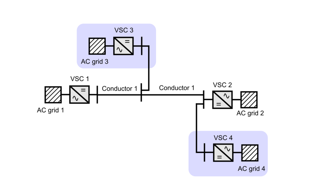
Figure 1 - Evolution of an existing HVDC link (VSC 1, VSC 2 and conductor 1) by connecting to additional converter terminals (VSC 3 and VSC4)
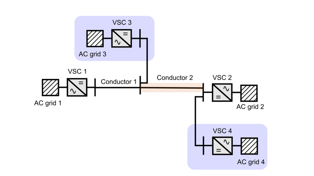
Figure 2 - Replacement of a part of Conductor 1 by Conductor 2 (with more power transmission capability)
Another option is to install a second conductor in parallel with the existing one (see Fig. 3). This approach reduces the cost compared to the first one, but it brings other challenges. The first one is that the current distribution between the two conductors cannot be controlled, since it depends on the resistance relation between them. The electric resistance depends not only on cross-section, conductor material, etc. but also on the conductor temperature. Then, it is not a constant parameter. This means that by installing a cross-section that can handle the increment of power, it is not possible to guarantee that the power distribution among conductors will comply with the desired power sharing. That is why, when a conductor in parallel is required, the best approach is to install a second conductor equal to the first one, to ensure equal power sharing between the two conductors. However, this may lead to install an oversized cross-section. Details on operation of cables in parallel are given in Section 2 of the paper.
This work proposes a third option, which consists in installing a second conductor in parallel with the existing one and a power flow controller (PFC) connected between the two conductors and the common terminal (see Fig. 4). This PFC, also known as current flow controller (CFC) is a medium voltage power electronic converter that can insert variable voltages in series with each conductor, thus, actively controlling their current distribution [5] [6]. This solution provides additional degrees of freedom to control the current sharing between the two conductors and may eventually reduce the cross-section requirement of the second conductor compared to the option of two conductors in parallel for the same total current. In this paper, a first economic assessment of the proposed reinforcement solution is provided. Firstly, the problem of the uncontrolled power distribution in two parallel conductors is explained, while detailing the model used in the study. Secondly, the solution of using the PFC connected between the two parallel conductors is presented, illustrating the model of the converter. After, the work details the methodology to compare the previous solutions and the cost hypothesis to conduct the economic assessment. Then, a case study is used to compare the two solutions and assess the economic interest of the solution with PFC. Finally, the conclusions of the work are summarized.
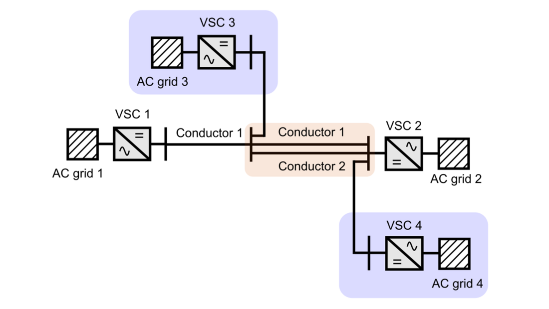
Figure 3 - Installation of Conductor 2 in parallel with a part of Conductor 1 to increase the power transmission capability
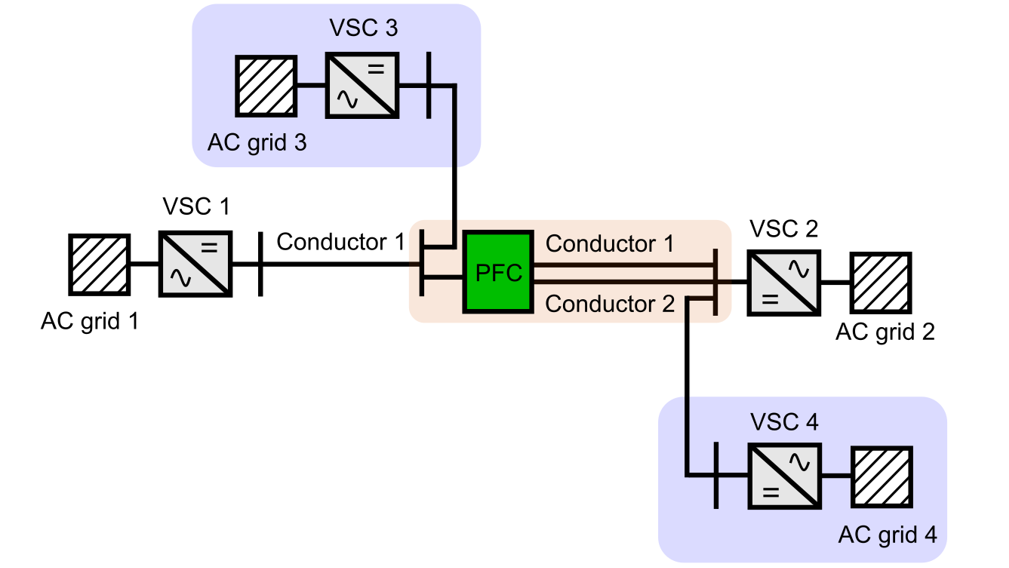
Figure 4 - Installation of Conductor 2 in parallel with a part of Conductor 1 (to increase the power transmission capability) and a PFC between both conductors to control the current distribution
2. Operation of cables in parallel
For the sake of simplicity, this works focuses on submarine cables as conductors, meaning that the models presented here and the following economic assessment are based on this assumption. However, an analogous work could be conducted if considering underground cables, overhead lines or a mix of them (the increase of current capability of an overhead line thanks to an additional underground cable in the same corridor).
As mentioned previously, during the upgrade or reinforcement of an HVDC system, it may be necessary to increase the power transfer capability of an already installed cable 1 from to
. A solution can be the installation of a second cable (cable 2) in parallel to be able to transmit the power increment
. Fig. 5 shows the initial state, with cable 1 capable of transmitting a power
between terminal A and B. Fig. 6 presents the system after the installation of cable 2 in parallel.

Figure 5 - Two HVDC terminals interconnected by a cable rated for a power Pa and transmitting the same power

Figure 6 - HVDC system of Fig. 5 after upgrading the system by installing another cable in parallel to transmit a total power Pf =Pa +∆P
As it is shown in Fig. 6, the total power being transmitted is but the power distribution between the two cables cannot be directly controlled since it depends on the resistance relation between the two conductors. Therefore, if a cable 2 is installed with the power rating of the upgrade (
), it cannot be ensured that cable 1 will transmit
and cable 2 will transmit
, as shown in Fig. 6. The rating of cable 2 will need to be higher than the power value of the upgrade (cable 2 rating ≥
), as it is demonstrated later in this paper.
The cable model used in this work is based on [7] and computes the resistance of a generic conductor as (1).
(1)
where, L is the length of the conductor, R0 is the DC resistance at 20°C per unit of distance, α20 is the resistivity variation coefficient at 20°C that depends on the material type, T is the measured temperature and Tref is the reference temperature (20°C). R0 depends on the cross-section and material of the conductor. To perform the analysis, the R0 of several cross-section are evaluated (obtained using the methodology in [7]) and a curve is fitted to get an analytical expression of R0 as a function of the cross-section and the conductor material.
The thermal model of the cable considers the physical dimensions and thickness of the different layers to compute an equivalent thermal resistance per km, Rth. The value of Rth is estimated from considering the thermal resistance of the conductor to the sheath, the sheath to the armour, the outer layer of the cable and finally the cable surface to the surrounding [7]. It takes into account that the cable is buried into the seabed and the value of thermal resistance considers the effect of the surrounding soil, but assuming that it is constant along the entire connection. An analytical expression of Rth is obtained as a function of the cross-section, same as for the DC resistance.
Finally, an expression to obtain the required cross-section to transmit a certain current without overheating the cable is also obtained following the same approaches than for the DC resistance and the thermal resistance.
The previous analytical expressions employed in this work for the DC resistance, thermal resistance, and the cross-section are given in the Appendix.
Fig. 7 presents a scheme of the two cables in parallel with their associated parameters and variables, that is employed to perform the comparative analysis of this paper.
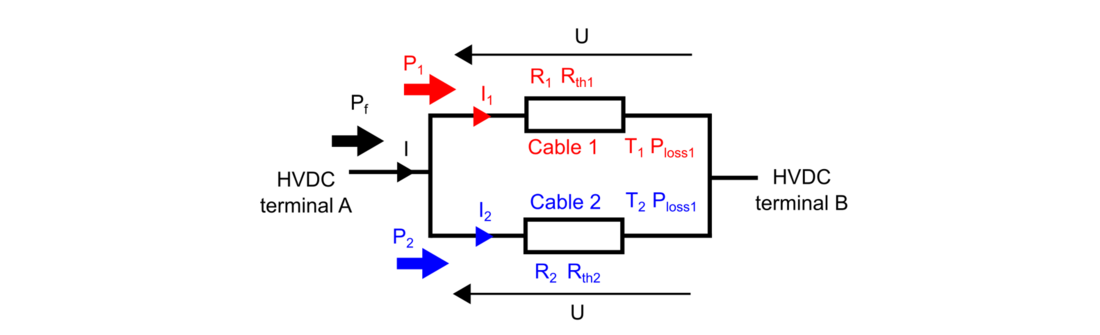
Figure 7 - Model of two cables in parallel to provide a power reinforcement into an existing HVDC system
Fig. 7 shows the two cables in parallel with the powers (P1, P2) and currents (I1, I2) that circulate through each one of them. The electric resistances (R1, R2 ), the thermal resistances (Rth1, Rth2) the temperatures (T1, T2) and the power losses (Ploss1, Ploss2) of each conductor are also illustrated.
Due to the parallel connection, their voltage drop (U) must be the same, which yields to (2).
(2)
Knowing that , the current distribution at each conductor can be calculated as in (3).
(3)
And then, the power losses at each cable can be assessed using (4) and (5).
(4)
(5)
The previous equations show that if R1<R2, cable 1 will concentrate more current and at the same time it will have higher losses.
The temperature of each conductor will depend on its power losses, the thermal resistance and the ambient temperature as shown in (6) and (7).
(6)
(7)
By combining (4) with (6) and (5) with (7) it is possible to see that considering the previous assumption R1<R2, if assuming equal thermal resistances (Rth1 = Rth2), T1 will be higher as shown in (8) and (9).
(8)
(9)
If similar thermal resistances are considered, the higher temperature will be mainly dictated by the higher power losses value. This could be the case of cables for example, where even when having different cross-sections, the values of thermal resistances are similar (they are mainly influenced by the nominal voltage, because of the insulation layers). Equations (8) and (9) express the temperature of each cable, but the resistances depend on those temperatures as well according to (1). The previous system of equations is solved numerically due to the difficulty to find an analytical formula.
Based on the previous analysis, the cable with the lower resistance will concentrate a higher amount of power (current) and assuming similar thermal resistances, it will operate close to its maximum temperature, when the total power transmission is . On the other hand, with the previous considerations, the cable with the higher resistance will operate at a temperature lower than the maximum (transmitting less power than its rating), which means it will be operated in a derated/underused mode.
If both conductors are equal, they will have the same resistance and thermal resistance, which leads to equal power distribution. In that situation, the previous problem does not exist.
3. Proposed solution with PFC
In order to solve the problem of uncontrollable current distribution in parallel cables, the use of PFC is proposed in this work. PFCs are medium voltage power electronic converters originally meant to control the current distribution in meshed HVDC systems [6]. In those kinds of systems, there is more than one path for the current to circulate from one terminal to another, meaning that the current distribution between the paths is imposed based on the resistance relation. In such case, some conductors may be overloaded, while others in the grid are underused, but the overall power transmission cannot be increased [5]. It can be seen that this situation is analogous to the problem of cables in parallel.
The PFCs can be understood as the equivalent of flexible AC transmission systems (FACTS) but applied to DC [8]. They provide additional degrees of freedom to control the power flows. In the literature, many converter topologies have been proposed to act as PFCs: series switching resistors [9], full power converters connected between poles [10] and variable voltage sources inserted in series with one line or with several lines [11], [12]. PFCs based on inserting series voltages sources in several lines have the advantages of not relaying in AC transformers to be connected to the AC side. Besides, by inserting voltages in series, with few kV it is possible to redirect hundreds or thousands of A [6]. This work considers the previous type of PFC to be connected to cables in parallel. By inserting voltages in series with the two cables it is possible to redirect part of the current from the overloaded cable to the underused one. By comparing this application to the meshed HVDC system, in cables in parallel the constraint in bidirectionality of the currents is smoothed, since the current can change the direction in both cables, but not exclusively in one. Whereas in a meshed HVDC system, the current bidirectionality of the cables may depend on the complexity of the DC grid, leading to more possibilities, thus probably to more complex PFCs.
Fig. 8 shows a PFC based on the topology presented in [13], connected between two cables in parallel. This converter structure allows to control the current between the two cables when they are in the same direction of the arrows in Fig. 8. The series voltages that the device applies must be in the same direction than the arrows in Fig. 8. If the current or the voltages are to be reversed, a more complex structure from [13] can be employed.
The PFC can be modelled as two voltages sources inserted in series with the parallel cables (see Fig. 9). The power extracted from one cable is injected into the other one (ensuring that , if neglecting the power losses).

Figure 8 - Two cables in parallel with a PFC connected between them and terminal A
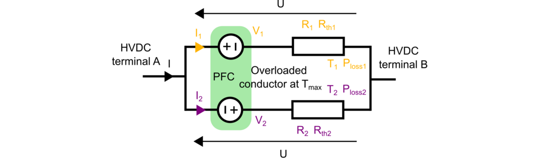
Figure 9 - Model of the two cables in parallel and the PFC as two voltage sources
By inserting series voltages, the currents circulating through the conductors can be controlled, and knowing the thermal resistance and the ambient temperature allows to regulate the temperature of each conductor.
It is expected that the PFC will not operate constantly. For low total powers being transmitted, if none of the cables achieves the maximum temperature, the PFC remains bypassed. During this situation, the model of the system is equivalent to the one in the previous section (see Fig. 7).
When one of the cables reaches the maximum temperature, as a consequence of transmitting its nominal current, the PFC is activated and it maintains such cable at the maximum temperature (transmitting the nominal power), while redirecting any power increment through the underused cable. Then, the model of the PFC and the parallel cables is defined by the following equations. For the sake of simplicity, the equations in this section represent the system assuming that cable 1 gets overloaded before cable 2, thus, the PFC controls cable 1 to the maximum temperature Tmax. The equations describing the control of cable 2 at Tmax are not shown here, but they are analogous. The temperature and power loss of cable 1 are shown in (10) and (11), respectively.
(10)
(11)
The current circulating through conductor 1 includes the temperature dependency in R1 (12).
(12)
The current of the conductor 2 can be calculated as (13).
(13)
Then, the power equivalency in the PFC is expressed in (14) as a function of K.
(14)
The temperature of conductor 2 is illustrated in (15).
(15)
Rearranging the previous expression, the temperature of the conductor 2 can be obtained as shown in (16).
(16)
After, the power losses in conductor 2 can be calculated using (17).
(17)
The electric resistance of conductor 2 depending on the temperature is shown in (18).
(18)
In (19) the same voltage drop in both conductors is imposed, which allows to find the applied voltages by the PFC.
(19)
By substituting (12)-(14) and rearranging, it leads to (20):
(20)
Then, by using (14), it is possible to obtain (21).
(21)
It is possible to solve analytically the previous system of equations.
4. Methodology
In order to assess the interest of the solution with PFC, it is assumed that a power upgrade of a certain HVDC cable is required. Two solutions are compared: Solution 1 with the installation of a second cable in parallel; and Solution 2 with the installation of a second cable in parallel and a PFC connected between them. The aim of the upgrade is to transmit the same total power, but as mentioned in Section 2, the installation of a PFC may provide a reduction in the required cross-section of the second cable of Solution 2 compared to the second cable of Solution 1. By introducing a simple cost model of the cables based on CAPEX and OPEX, it is possible to assess if the reduction in the cross-section in Solution 2 is relevant or not.
4.1. Cost model
The cost of the cables (CAPEX) is expressed as:
(22)
where, Cinstallation is the installation cost per unit of distance and Csupply is the cost of supply per unit of distance given by:
(23)
where, and b are two coefficients, VDC is the nominal DC voltage that the cable withstands and S is the cross-section of the conductor. Since cable 1 is the same in both Solution 1 and 2, Ccapex includes only the cost of the second cable for both solutions.
The cost of the losses (OPEX) is expressed as:
(24)
where, Tproject is the lifetime of the project in which the losses are calculated; Cenergy is the cost of energy; LF0% is the percentage of the total time working at 0 power in pu; LFX% is the percentage of the total time working at X% (partial power, between 0 and 100%) in pu; LF100% is percentage of the total time working at full power in pu; P0% are the sum of the power losses of cable 1 and cable 2 when transmitting 0 power, which is assumed here to be 0; PX% are the sum of the power losses of cable 1 and cable 2 when transmitting X% of the nominal power (partial power operation); P100% are sum of the power losses of cable 1 and cable 2 when transmitting the nominal power. In (24), a link working at three different power levels is considered for this study, but any power profile could be applied.
The losses of the PFC for Solution 2 are not included in the cost calculation since it is assumed that they are negligible (an order of magnitude lower compared to the losses in cables) [6], [11].
The total cost of each solution ( for Solution 1 and
for Solution 2) is expressed in (25) and (26), respectively:
(25)
(26)
The CAPEX of Solution 1 will be equal or higher than the one of Solution 2 () since the PFC can reduce the required cross-section of cable 2. However, the OPEX of Solution 2 will be equal or higher than Solution 1 (
), because the PFC increases the losses when modifying the currents and the reduced cross-section of cable 2 in Solution 2 also leads to higher losses for the same total current.
The PFC cost is difficult to estimate since there is no commercial product or real scale prototype. Although, the main power electronic components of the PFC are known and their cost could be estimated, the PFC total cost will be impacted by other factors, such as isolation, cooling, protection (bypass switches for overcurrent), switches to bypass/insert, control equipment, installation constraints (onshore or offshore). Many of the previous factors are only known by manufacturers, thus, the building of a cost model for the PFC is left as a perspective of this work. Additionally, not only the values of voltage and current in steady state should be considered to size the PFC, but also the possible transients in the system, which may increase the final cost. That is why it is chosen not to include the PFC cost in Solution 2. Instead, a break-even cost of the PFC ( ) is defined in order to assess the attractiveness of Solution 2.
is calculated as shown in (27) by resting the total cost of Solution 2 (excluding the PFC) from Solution 1.
(27)
If this is positive, it implies that Solution 1 is more expensive than Solution 2 (without including the cost of the PFC itself). This positive value of
gives a profitability threshold or break-even cost, setting an upper limit to the cost that the PFC could have and still make Solution 2 less expensive than Solution 1. The higher the value of
, the higher the difference of cost between the two solutions (excluding the PFC), what implies that the profitability threshold is higher and the PFC real cost could be higher and still make Solution 2 more economically interesting. In general, the higher the
, the more interesting is Solution 2.
On the contrary, if the calculated value of is negative, it means that Solution 2 (without including the cost of the PFC) is already more expensive than Solution 1. In that case, Solution 2 is not interesting from an economic point of view.
The is divided by the power rating of the PFC, PRPFC, leading to
.
provides a break-even cost of the PFC per unit of PFC power. This
can be compared with the cost/MW of similar HVDC power electronic converters. Assuming that similar converters would have similar cost/MW, if the
is higher than the known values of cost/MW of similar converters, it may imply that the PFC can be built and Solution 2 (including the real cost of the PFC) would be less expensive than Solution 1. Therefore,
is used as an indicator of the economic interest of the Solution 2. The higher
, the more economically interesting Solution 2 is.
4.2. Workflow
The workflow of the methodology to compare the two solutions is presented in this subsection.
The actual power of the link, , and the final power of the link, Pf, are defined.
is used to define the cross-section of cable 1, which is common to both Solution 1 and 2. Equations (35)-(36) are used to obtain the cross-section as a function of the current through the cable.
The final power of the link, Pf, is used to calculate the required cross-section of cable 2. The way to estimate the required cross-section depends on each solution.
In Solution 1, an iteration is performed to obtain the smallest cable 2 cross-section that ensures T1, T2<Tmax. Due to the current distribution according to the relation between cables resistances, if the cables are different, one of them will reach before the maximum temperature and the other will be underused (it is not possible to ensure that cable 2 will transport ). Cable 2 cross-section is progressively increased and the system of equations (8)-(9) solved, until the temperatures of both cables are below Tmax . Then, the first cross-section that complies with that is selected for cable 2. When solving the system of equations, the currents and power losses of the cables are also obtained.
In Solution 2, the procedure is more straightforward since the PFC can ensure that both cables work at the maximum temperature when transmitting the final power. Therefore, the cross-section of cable 2 can be obtained using (35)-(36), knowing it will carry a power of . Once the cross-section is selected, the equations in Section 3 can be used to calculate the final temperatures, currents, powers and voltages inserted by the PFC.
Once all the physical parameters are determined for each solution, the cost model described in Section 4 is employed to quantify their cost. The previous methodology is applied not to a single final power but to several final powers between and
to assess the advantages of Solution 2 assuming a range of possible final powers in the upgrade.
Fig. 10 shows a diagram with both Solution 1 and Solution 2, where the cable 1 has the same cross-section for both and cable 2 is different, as explained before. In Fig. 11, a flowchart of the methodology to compare the economic interest of both solutions is illustrated.
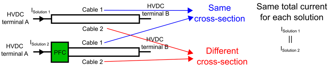
Figure 10 - Diagram representing the two solutions to reinforce and existing HVDC cable (Solution 1 on top, Solution 2 on the bottom)
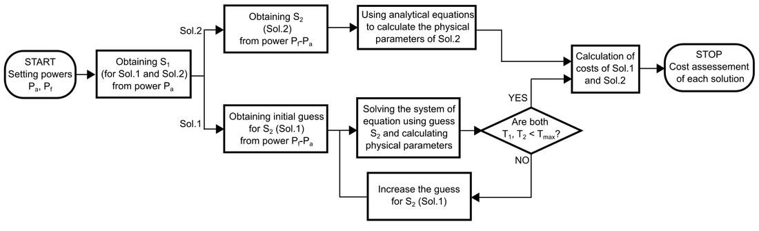
Figure 11 - Flowchart of the methodology to assess the cost of each solution

5. Case study
This section presents the results of applying the methodology explained in Section 4. The initial power of the link is set at 700 MW, while the final power Pf to be transmitted changes from 700 MW to 2000 MW (
). The link is considered to be a symmetric monopole with a voltage of ±320 kV. The cables are assumed to be made of Cu conductor and the distance ? is 200 km. The commercially available cross-sections are assumed to be: 500, 600, 800, 1000, 1200, 1400, 1600, 1800, 2000, 2200, 2500, 2600, 2800 and 3000 mm². The physical and costs parameters used in the case study are illustrated in Table I.
| Parameter | Symbol | Value | Units |
|---|---|---|---|
| Maximum temperature of the conductor
| Tmax | 70 | °C |
Ambient temperature | Tamb | 20 | °C |
Resistivity coefficient of Cu at 20°C | 0.00403 | K-1 | |
Project lifetime | Tproject | 15 | years |
Load factor at 0 power | LF0% | 0.1 | - |
Load factor at 50% power | LF50% | 0.4 | - |
Load factor at 100% power | LF100% | 0.5 | - |
Energy cost | Cenergy | 150 | €/MWh |
Installation cost | Cinstallation | 400.5 | k€/km |
Coefficient a (supply cost) | 1.0287 | k€/(kV·km) | |
Coefficient b (supply cost) | b | 0.333 | k€/(mm²·km) |
5.1. Cross-section selection results
The results concerning the selection of the cross-section for both Solution 1 and 2 are shown in this section.
The following figures present the result as a function of different final powers Pf (power transmitted in the horizontal axis) considering the same initial power of 700 MW. The final powers of
, twice
and
(which represents the maximum value of final power considered, 2000 MW) are highlighted with a vertical dashed line on each graphic. Fig. 12 presents the results showing the cable cross-section requirement (see Fig. 12(a)) and the temperature of both cables (see Fig. 12(b)).
In Fig. 12(a), the section of Cable 1 (S1) in both Solution 1 and 2 is constant for each final power since it is defined by the initial power , the cable that is already installed before the upgrade. Regarding the cross-section of Cable 2 (S2) for both solutions, initially it is constant when increasing the power transmitted since the minimum available cross-section is 500 mm². This means, that until a certain final power, cable 2 is oversized in both solutions. In Solution 1, S2 increases for lower final powers, since the PFC in Solution 2 regulates the current distribution, it is possible to transmit the same power with a smaller cross-section, optimizing the use of the two cables. When the final power approaches to 2
, S2 in both solutions starts to converge, until they reach 2
, where they have the same value. This happens because at 2
, the required cross-section for cable 2 in both solutions will be the same as cable 1, since the power transmitted is twice the initial power. At this point, the PFC has no interest because the currents are distributed equally between both cables, and they have the same temperature as shown in Fig. 12(b). S2 in Solution 2 is always equal or lower than S2 in Solution 1, and this difference increases the further the final power goes away from 2
. It can also be noticed that in Solution 1, S2 reaches the maximum available cross-section (3000 mm²) for lower values of Pf than for Solution 2, which restricts the maximum final power (to 1700 MW approximately). While in Solution 2, thanks to the PFC, the use of both cross-sections is optimized, and the maximum transmitted power can reach approximately 1900 MW. In Solution 1, a third cable would be used to reach this total transmitted power. The maximum final power of 2000 MW cannot be transmitted with two cables neither in Solution 1 nor Solution 2, since both cables achieve a temperature of 70ºC.
Fig. 12(b), shows the temperatures of the conductor in each cable and for each solution. Initially, the temperatures are the same for cable 1 in both solutions and for cable 2 in both solutions. The PFC is not used since all cables remain below Tmax. At Pf around 1050 MW, cable 1 in Solution 1 reaches Tmax, which requires an increase of the cross-section of cable 2 for transmitting higher powers. However, in Solution 2, the PFC controls cable 1 at Tmax, while redirecting the current through cable 2, so that, increasing T2. The saw-tooth waveform is explained because each time the power is increased may provoke an increase in the cross-section, as well. However, the immediate power level afterwards may not require the whole rating of the new cross-section, thus, the maximum temperature is not achieved. The temperatures of the four cables are the same at 2 and for higher powers, they start to diverge again.
Fig. 13(a) presents the total power losses in both cables for both solutions and Fig. 13(b) shows the currents circulating through each cable and solution. Initially, the currents are equal between solutions as shown in Fig. 13(b) since the PFC remains bypassed. When the final power reaches 1050 MW, the PFC (Solution 2) keeps the current through cable 1 at its rating, while increasing the current through cable 2. In Solution 1, the current of cable 1 is also kept at its rating (it gathers most of the current since it has a larger cross-section than cable 2, so less resistance). However, after 2 , cable 2 in Solution 1 has a larger cross-section (see Fig. 12(a)) and starts to gather more current than cable 1. After this power, in Solution 1, I2 keeps increasing, while I1 is reducing (meaning that cable 1 becomes more underused). Fig. 13(a) shows that the total losses are equal in both Solution 1 and 2 when the PFC is bypassed, and the cross-sections of the cables are the same. Nevertheless, the use of the PFC in Solution 2 brings an increase in the total losses, since the current distribution is different from the natural current distribution that ensures minimum losses and a smaller cross-section for cable 2 is used (with more resistance).
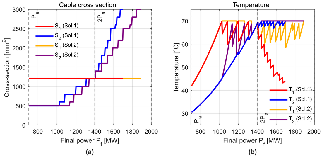
Figure 12 - Results of the cross-section selection. (a) Cross-section requirement for each cable and solution. (b) Temperature of the conductor for each cable and solution
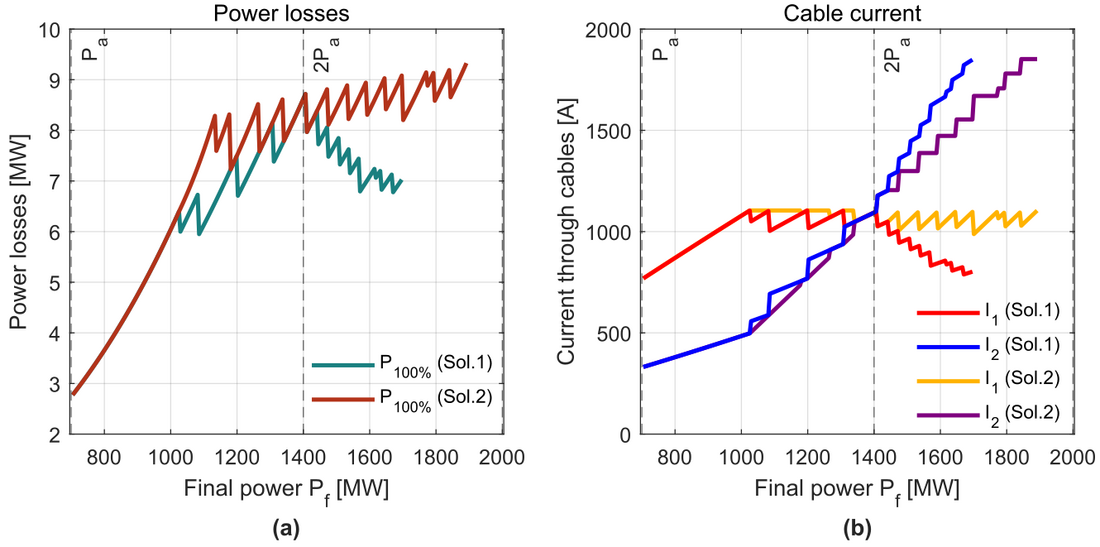
Figure 13 - Results of the cross-section selection. (a) Total power losses at nominal power for each solution. (b) Current circulating through each cable and for each solution
Fig. 14(a) illustrates the required series voltages that the PFC must apply with each cable in Solution 2. The PFC rating is then shown in Fig. 14(b). When the PFC is bypassed, the applied voltages are 0 in both cables as seen in Fig. 14(a). Then, after a final power level of 1050 MW, the required voltages increase. They are positive until 2, since the PFC needs to apply a voltage that reduces the current through cable 1 and increases the current through cable 2 (according to Fig. 9), because the cross-section of cable 1 is larger than the cross-section of cable 2. At 2
, there is no need of PFC (voltages are 0) and for higher powers, the situation is inversed. Cable 1 has a smaller cross-section than cable 2, which leads the PFC to apply negative voltages (according to Fig. 9) to reduce the current of cable 2 and increase the current of cable 1. Fig. 14(b) shows that the rating of the PFC increases when it goes away from 2
, with the exception of low powers, when it is not required.
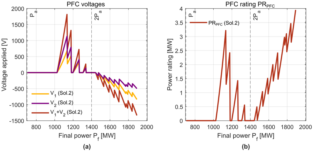
Figure 14 - Results of the cross-section selection. (a) Series voltages inserted by the PFC in Solution 2. (b) Power rating of the PFC for each final power in Solution 2
5.2. Results for a selected final power of the link
To detail the previous results for a specific upgrade example, the data of final power 1600 MW is extracted in this section. The required cross-sections are identified for the expected final power and then, they are kept constant while performing a power sweep from 0-1600 MW. This analysis allows to check the variables of the system when it is not working at full power.
For the final power of 1600 MW, the required cross-sections are shown in Table II. Fig. 15 presents the results showing the temperature, total power losses, currents and PFC voltages.
| Solution 1 | Solution 2 | |
|---|---|---|
Cable 1 | 1200 | 1200 |
Cable 2 | 2500 | 2000 |
Fig. 15(a) shows how, T2 rises faster than T1 and reaches Tmax since the cross-section of cable 2 is larger than cable 1 in both solutions. Around 1520 MW, the PFC is activated and starts to control T2 at Tmax while T1 increases when increasing the power. At 1600 MW, T2 in Solution 1 is almost Tmax, while T1 remains much lower (underused cable).
Fig. 15(b) depicts the total losses in both cables for each solution (the losses of the PFC are assumed to be negligible). It can be noticed that the losses of Solution 2 are higher than the losses of Solution 1 even when the PFC is not used (it is bypassed until the power is approximately 1520 MW). The cross-section of cable 2 in Solution 2 is 2000 mm², while in Solution 1 is 2500 mm², so by transmitting the same total power, the higher resistance of cable 2 in Solution 2 induces a higher level of losses. The difference between the losses of both solutions increases when increasing the power.
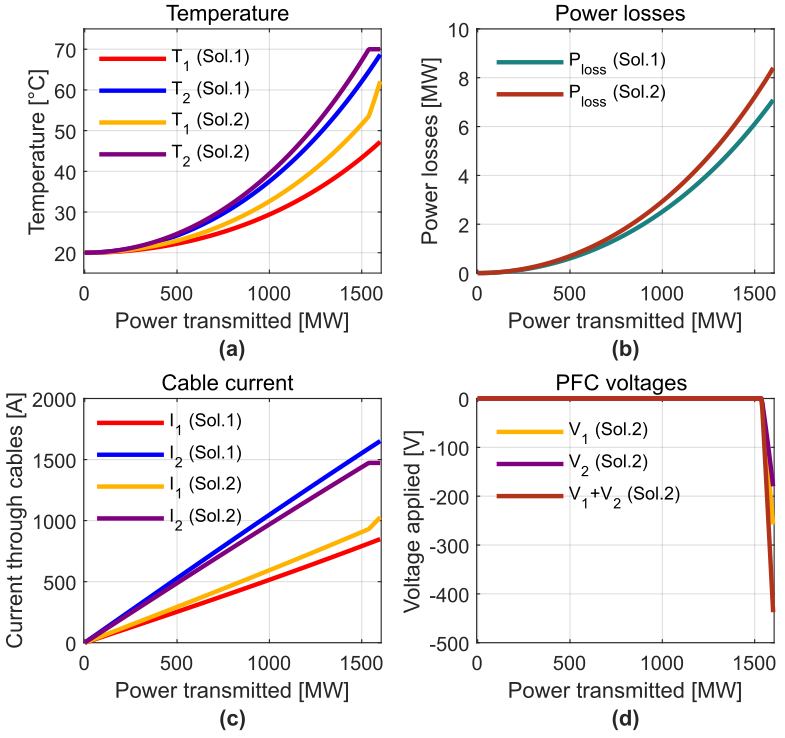
Figure 15 - Results considering the cross-sections of final power 1600 MW for both solutions. (a) Temperature. (b) Power losses. (c) Currents through cables. (d) PFC voltages
Fig. 15(c) presents the currents circulating through the cables. Cable 2 in both solutions gathers more current, since the cross-section is larger. At 1520 MW, it is possible to see how the PFC controls the current of cable 2 (Solution 2) at the maximum rating.
The voltages inserted by the PFC and its sum (V1+V2) are illustrated in Fig. 15(d). As mentioned before, for most transferred powers, the PFC remains bypassed, and the inserted voltage is 0. This means that even if a PFC is required for Solution 2 to use a reduced cross-section of cable 2, the operation of the device is only needed when the power transmitted is between 1520-1600 MW.
Fig. 16 and Fig. 17 show the schematics of both solutions for final power of 1600 MW and operating at the nominal power, illustrating temperatures, power, currents and voltages.
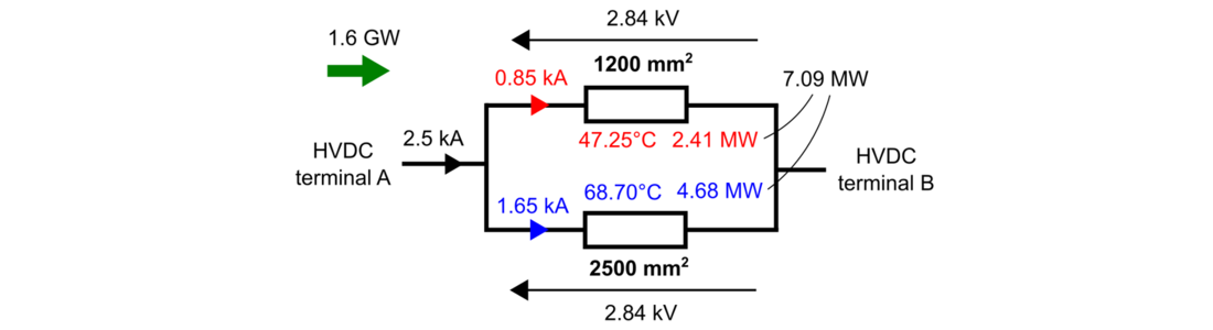
Figure 16 - Solution 1 at nominal power 1600 MW
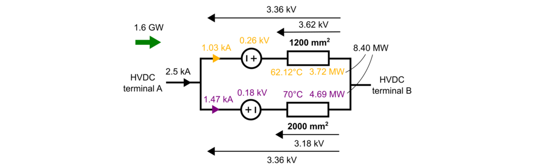
Figure 17 - Solution 2 at nominal power 1600 MW
The electric and thermal resistances of cables in Fig. 16 and Fig. 17 are presented in Table III.
| Parameter | R1(T1) [Ω] | R2(T2) [Ω] | Rth1 [K/MW] | Rth2 [K/MW] |
|---|---|---|---|---|
Solution 1 | 3.34 | 1.72 | 11.33 | 10.40 |
Solution 2 | 3.52 | 2.16 | 11.33 | 10.67 |
5.3. Cost assessment results
Fig. 18 presents the results of the cost assessment, by comparing the costs of Solution 1 and 2. In each graphic, there is a shaded area in purple that represents the final powers, in which Solution 1 cannot transmit the desired power since the maximum commercially available cross-section is used. On the contrary, for those final powers in the shaded area, Solution 2 allows to transmit the desired power by optimizing the use of both cable 1 and 2 thanks to the PFC. For higher powers after the shaded area, neither Solution 1 nor 2 can transmit the desired power. This is based on the hypothesis that the link is upgraded by a second cable in parallel, the use of further cables in parallel is not considered in this work.
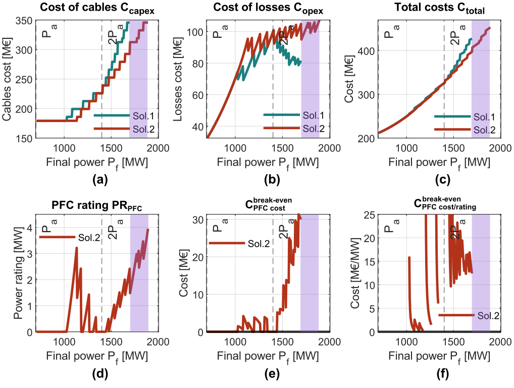
Figure 18 - Results of the cost assessment. (a) Cost of cables. (b) Cost of power losses. (c) Total costs. (d) PFC power rating. (e) PFC break-even cost. (f) PFC break-even cost divided by the PFC rating
Fig. 18(a) shows the cost of the cables (considering the supply and installation cost as explained in Section 4.1.). The results are proportional to the cross-section requirement in Fig. 12(a), showing that Solution 2 is especially interesting after 2 and very interesting for the powers in the shaded area, since with Solution 1, it is not possible to transmit the desired power.
Fig. 18(b) presents the cost of losses of both solutions. The results are similar to Fig. 13(a), since with Solution 2, the losses are always equal or higher, due to the reduced cross-section of the cable 2 and the operation of the PFC.
The total costs are shown in Fig. 18(c), by summing the cost of cables and the cost of losses. It can be seen that the higher cost of losses of Solution 2 is compensated by the savings in the cross-section of cable 2. This makes Solution 2 more economic than Solution 1, especially after 2 and it increases with the final power. As said before, in the shaded area, Solution 2 is even more interesting, since Solution 1 cannot transmit the desired power.
Fig. 18(d) depicts the rating of the PFC for each final power in Solution 2. As it can be seen, the rating increases the further the final power goes away from 2, since the PFC has to apply higher voltages because the cross-sections of cable 1 and cable 2 become more different. The maximum rating is 4 MW for a final power of almost 2000 MW, since the rated current flows through the device, but it only inserts voltages lower than 1 kV.
In Fig. 18(e), for each final power is depicted.
is the rest between the total cost of Solution 1 and the total cost of Solution 2. If this value is positive, means that Solution 2 may be interesting, since its cost without including the PFC is lower than the cost of Solution 1. Then, this value gives an upper limit for the cost of the PFC device. In case the value is negative, Solution 2 is not interesting because, without considering the cost of the PFC, the cost of Solution 2 is already higher than Solution 1. It is possible to see that for low final powers, the value is negative (only positive values are depicted in the graphic), while for values higher than 2
,
rises up to 30 M€. The shaded area in the graphic depicts no cost since it is not possible to obtain the numerical value because in Solution 1 it is not possible to reach that final power (a third cable in parallel would be required). Although a value of
is not provided in this area, Solution 2 is more interesting economically than Solution 1, as it allows to transfer the power using two cables in parallel, whereas for Solution 1, a third one should be installed (something that the model does not contemplate).
In Fig. 18(f) depicts (the previous
divided by the rating of the PFC, PRPFC). This graphic gives an indicator of how much can the PFC cost (in M€/MW) to make Solution 2 economically interesting compared to Solution 1. Neither the points where the PFC has 0 rating nor the points where
is 0 or negative values are plotted in Fig. 18(f), so that the curve is not continuous. Additionally, due to the division by values close to 0 (PRPFC is almost 0 in some points, see Fig. 18(d)), the curve for Solution 2 presents important peaks up to 300 M€/MW, which are not shown in the graphic. They are not considered to be relevant, since they are happening in very narrow regions of powers, something that might not be interesting from a practical perspective. For the region of powers higher than 2
, the
varies between 10-24 M€/MW. Additionally, the shaded area represents the final powers in which Solution 2 is also interesting, since the power transfer cannot be done considering Solution 1 with two cables. Taking into account that an MMC station cost is in the order of magnitude of 0.1 M€/MW, the previous
shows that the device could be built and Solution 2 would still imply savings compared to Solution 1.
5.4. Sensitivity analysis
This section provides a sensitivity analysis of the previous cost assessment, in order to identify how a variation of some of the parameters affects the , so the economic interest of Solution 2. Five cases are considered (Case 1 to 5), in which four parameters are changed with respect to the reference result of Section 5.3. These parameters are the link length L , the cost of energy Cenergy , the power profile (partial power X ), and the lifetime of the project Tproject. The effect of changing the different parameters on the
is illustrated in Table IV.
| Cost of energy Cenergy [€/MWh] | Length L [km] | Partial power X [%] | Project lifetime Tproject [years] | [M€/MW] | |
|---|---|---|---|---|---|
| Reference | 150 | 200 | 50 | 15 | 10-24 |
| Case 1 | 75 ↓ | = | = | = | 17-35 ↑ |
| Case 2 | = | 400 ↑ | = | = | = |
| Case 3 | = | = | 100 ↑ | = | 3-12 ↓ |
| Case 4 | = | = | = | 30 ↑ | 1-5 ↓ |
| Case 5 | 100 ↓ | = | 80 ↑ | 20 ↑ | 7-22 ↓ |
The reference case, shown in Fig. 18(f), shows that the is in the range of 10-24 M€/MW for final powers higher than
, without considering the spikes.
Case 1 presents the if the cost of energy is reduced to 75 €/MWh. Since Solution 2 has the inconvenient of increasing the losses compared to Solution 1, a reduction in the cost of energy is beneficial for Solution 2. Thus, the
reaches a range of 17-35 M€/MW, making Solution 2 more economically favourable.
Case 2 illustrates the effect of increasing the distance of the link up to 400 km. It can be seen that the modification leads to the same results as the reference, with the same . This is due to the fact that both the cost of cables and losses are doubled but the same happens for the rating of the PFC. The longer the distance, the higher the resistance of the cables, and the higher the PFC required voltage. Since the costs and the PFC rating are both proportional to the distance, the
is kept constant.
In Case 3, the power profile of the link is modified. The operation at partial power (during 40% of the time according to Table I) is increased from 50% to 100%. It means that the link operates 10% of the time at 0 power and 90% of the time at full of the power. This negatively impacts the interest of Solution 2, since it brings the same reduction in cable costs, but the cost of losses increases (more power is transmitted, thus more losses). Therefore, the decreases to the range of 3-12 M€/MW.
Case 4 shows the effect of increasing the project lifetime. It can be seen how the interest of Solution 2 decreases as the is reduced to a range of 1-5 M€/MW, though still being positive. This is a consequence of the increase of the cost of losses but keeping the same cost of cables.
Finally, in Case 5, several parameters have been modified: cost of the energy decreased, partial power and project lifetime increased. The reduction in the cost of energy increases the interest in Solution 2 by lowering the cost of losses, but the increase in the partial power and project lifetime have the opposite effect. The resulting is in the range of 7-22 M€/MW.
6. Conclusions
The reinforcement of conductors may be necessary when interconnecting existing HVDC systems, if the grid development plan did not consider the oversizing of the conductors for future upgrades. This work has presented an alternative to installing a conductor in parallel with an existing one to reinforce the power transmission of an HVDC system. The solution consists in installing a second conductor in parallel with an existing one and a PFC connected between them. Since the PFC is able to control the power distribution between the two conductors, a smaller cross-section for the second conductor can be selected, compared to the one considering two conductors in parallel without PFC. The paper introduces the electric and thermal model of DC submarine cables to be used in the study. Then, it shows the methodology to compare the two solutions: two cables in parallel with and without PFC. The analysed case study considers an initial transmitted power (through the first cable) and several final powers to be transmitted by the two cables, to assess the interest of the proposed solution for different final powers. The solution with PFC provides a reduction in the required cross-section of the second cable but it increases the power losses when transmitting the same power. The results show that for final powers higher than twice the initial power, the savings in the cost of the second cable compensate the increase in cost of operation (losses), making solution with PFC more economically interesting than the solution with two cables in parallel. The PFC cost is not included in the cost of the proposed solution, instead a break-even cost/power rating for the PFC that makes solution with PFC cheaper is obtained from the previous analysis. This cost/rating is lower than the cost/rating of an MMC station, outlining the economic feasibility of the device. The sensitivity analysis shows that the solution with PFC becomes more interesting for low project lifetimes, low cost of energy and a low load factor of the HVDC system. The analysis has been performed for submarine cables, but further works should assess the interest of the solution with PFC when using underground cables or overhead lines. Another perspective is a more advanced cost analysis (considering e.g., inflation, PFC impact on system availability, PFC cost model, etc.).
7. Appendix
The analytical expressions of the DC resistance, thermal resistance, and the required cross-section to transmit a certain current Imax are shown in (28)-(36). The cable cross-section (S) is expressed in mm² and the current in A, for a nominal DC voltage of the cable of 320 kV.
(28)
(29)
(30)
(31)
(32)
(33)
(34)
(35)
(36)
Acknowledgment
This work was funded by SuperGrid Institute, an institute for the energetic transition (ITE). It is supported by the French government under the frame of “Investissements d’avenir”, No. ANE-ITE-002-01.
References
- European Comission, "Offshore Renewable Energy Strategy," 2019. [Online] [Accessed 20 09 2021].
- D. Van Hertem, O. Gomis-Bellmunt and J. Liang, HVDC Grids: For Offshore and Supergrid of the Future, IEEE Press Series on Power Engineering. John Wiley & Sons, 2016.
- e-Highway2050, "Europe’s future and secure and sustainable electricity infrastructure," 2015. [Online] [Accessed 20 09 2021].
- Amprion, "Amprion connects climate protection by innovation," 2020. [Online] [Accessed 20 09 2021].
- E. Veilleux and B.-T. Ooi, "Power flow analysis in multi-terminal HVDC grid," in IEEE/PES Power Systems Conference and Exposition, Phoenix, USA, 2011.
- J. Sau-Bassols, F. Morel, S. Touré, S. Poullain and F. Jacquier, “Methodology to obtain the specifications and perform the sizing of a power flow controller for meshed HVDC grids,” in European Conference on Power Electronics and Applications EPE'21 ECCE Europe, Virtual, 2021.
- S. Gasnier, A. André, S. Poullain, V. Debusschere, B. Francois and P. Egrot, "Models of AC and DC Cable Systems for Technical and Economic Evaluation of Offshore Wind Farm Connection," International Journal of Electrical Energy, vol. 6, no. 2, pp. 64-73, 2018.
- O. Gomis-Bellmunt, J. Sau-Bassols, E. Prieto-Araujo and M. Cheah-Mane, "Flexible Converters for Meshed HVDC Grids: From Flexible AC Transmission Systems (FACTS) to Flexible DC Grids," IEEE Transactions on Power Delivery , vol. 30, no. 1, pp. 2-15, 2020.
- Q. Mu, J. Liang, Y. Li and X. Zhou, "Power flow control devices in DC grids," in IEEE Power and Energy Society General Meeting, San Diego, USA, 2012.
- D. Jovcic, "Bidirectional, High-Power DC Transformer," IEEE Transactions on Power Delivery, vol. 24, no. 4, pp. 2276 - 2283, 2009.
- C. Barker and R. Whitehouse, "A current flow controller for use in HVDC grids," in 10th IET International Conference on AC and DC Power Transmission, Birmingham, UK, 2012.
- J. Sau-Bassols, E. Prieto-Araujo, O. Gomis-Bellmunt and F. Hassan, "Series Interline DC/DC Current Flow Controller for Meshed HVDC Grids," IEEE Transactions on Power Delivery, vol. 33, no. 2, pp. 881-891, 2018.
- S. Touré, F. Morel and S. Poullain, "Power flow control device for controlling the distribution of currents in a mesh network". Patent EP3656030 B1, 2020.