Power generation by unhealthy photovoltaic modules
Authors
R. RAIMUNDO, I. CATARINO - NOVA School of Science and Technology, Portugal
A. COELHO, R. MARTINS - EDP Labelec, Portugal

Summary
Hotspots are one of many defects that can occur on degraded photovoltaic system, yielding a detrimental effect on the PV module production. Infrared thermography was used to detect and quantify the severity of hotspots. Temperature difference between overheated and healthy areas was assessed. Four PV modules were analysed, one of them presenting a hotspot.
A model for both healthy and unhealthy PV modules was developed, based on the single diode solar cell model and considering, exclusively, data-sheet parameters. To validate the model, the outputs for these working conditions were compared with the real outputs of the studied PV modules, which were previously measured and stored.
The relationship between the severity of a hotspot and its respective impact on the power generation of the PV module was studied and the consequent monetary loss can be assessed. Thermographic analysis was enhanced as an optimizing decision-aid tool for the operation of photovoltaic installations.
keywords
Infrared thermography - PV modelling - single-diode model - irradiance - temperatureNomenclature
a Diode’s ideality factor
G Irradiance
Gstc Standard Test Conditions irradiance
I electric current at PV cell’s terminal
I0 Diode’s saturation current
Id Diode's electric current
Impp Maximum power point current
Iph Photogenerated current
Isc Short circuit current
Ish electric current along Rsh
Istc Standard Test Conditions electric current
kB Boltzmann’s constant
KI Temperature coefficient for shortcircuit current
KV Temperature coefficient for open circuit voltage
NS Number of PV cell in the module
P Electric power
q Electron charge
RS Series resistance
Rsh Shunt resistance
T Temperature
Ta Ambient temperature
V Electrical voltage at PV cell’s terminals
Vmpp Electrical voltage at maximum power point
Voc Open circuit voltage
Vt Electrical thermal voltage
1. Introduction
A photovoltaic (PV) module can deteriorate over time due to the environmental conditions to which it is exposed, or in the manufacturing, transport and installation processes. This degradation can lead to a decrease in the performance of these photovoltaic systems, resulting in a variation in their energy production. For this reason, it is important to study the defects of photovoltaic modules, in order to minimize the energy loss and ensure a greater use and efficiency of this energy source. One of these possible defects is the presence of hotspots, which can be detected through a non-destructive test called infrared thermography, detecting the thermal energy emitted by objects, in the infrared region of the electromagnetic spectrum, and further transforming it into a visible image.
As the name hotspot suggests, there will be a region on the PV module where the temperature is higher than normal, and this can damage the solar cell or any other element of the panel. Hotspots usually appear as a consequence of different failure modes, such as breakages on the front glazing, internal cell problems and external shading, that can affect the solar cell properties, such as the p-n junction deformation, local shunts, presence of impurities and wafer resistance.
This work was developed under the Asset Inspection area of EDP Labelec, using real energy production data retrieved from the Sunlab Project. A thermographic analysis was then undertaken, in order to both identify and quantify the severity of the defect. To understand the effect of hotspots on the module and to predict the energy output of the PV modules, and respective loss of power generation, in a year scale, a model for both healthy and unhealthy PV modules was developed, based on the single diode solar cell model and considering, exclusively, data-sheet parameters. To validate the model, the outputs for these working conditions, for both healthy and unhealthy PV modules, were compared to the real outputs of the studied PV modules, which were previously measured and stored. This model predicts the module behaviour taking into account the influence of both temperatures and irradiance conditions. The developed model was tested using temperature and irradiance data from a weather station located next to the PV modules under study, for both healthy and unhealthy PV modules.
This article aims to relate the level of severity of a hotspot anomaly with its impact on the energy production of a PV module, evaluating the variation in energy production on modules with and without defects. Furthermore, a model that describes the electrical behaviour of a healthy photovoltaic module was adapted, through the simulation of several hypotheses, in order to model a module with a hotspot. It was used 2 years of data of energy production (power, current and voltage) of monocrystalline silicon modules (three modules in good condition and one module with a hotspot type defect) as well as data from a meteorological station (temperature, humidity, irradiance, precipitation, etc.), located very close to the modules. The datasheet information of the modules was also used. This analysis intends to develop a model to help PV asset management, helping to estimate and evaluate the impact of hotspots defects.
1.1. Infrared thermography applied to photovoltaic modules
Infrared thermography (IRT) is a method of determining the temperature distribution on the surface of an object by measuring the intensity of electromagnetic radiation in the infrared region. Using infrared cameras, the acquired images are converted into visible images, by assigning a colour to each energy level. These images are known as thermograms, where each pixel in the thermogram has a specific infrared radiation value, and the image contrast derives from differences in the temperature of the surface of the object under study. Currently, IRT has numerous applications, both at the level of research and development and at the industrial level. One of the applications is the inspection of photovoltaic modules to detect hotspots. The IRT technique can be applied to photovoltaic modules, and it is possible to use it both with and without sun exposure. One of the great advantages of this technique is that, being a non-invasive technique, it can be applied to modules in operation, being possible to indicate the presence of defects in areas where the radiated temperature is higher than the neighbourhood.
In a photovoltaic module, the radiation that hits the cells can be converted into current, heat and reflected radiation. In cell regions that contain defects, less radiation will be converted into current, most of which is converted into heat and eventual reflection, which causes this region to heat up. In a photovoltaic module, the temperature that is detected by infrared camera is not only determined by the radiation emitted by the module itself, but also by radiation from the neighbourhood, typically sky and clouds and the surrounding environment. For the temperature measurements to be representative of the module under study, it is necessary to consider the expected data on the emissivity of the photovoltaic module, the reflected radiation, the air temperature, the humidity and the distance between the module and the camera. A crucial condition for obtaining quality infrared images is that the environmental conditions are stable during measurements. Common environmental changes that affect the quality of infrared images from modules are the cloudy overlapping of the sunlight, which causes a rapid variation in irradiance. Another important aspect to take into account when performing IRT measurements is that the glass that covers the module is a very reflective material, this reflection being dependent on the wavelength. Thus, to prevent the glass cover of the photovoltaic module from influencing the measurements, the camera angle must be varied with angles between 5º and 60º [1] (0º being the angle perpendicular to the plane of the photovoltaic module).
1.2. Hotspots
Hotspots are regions of the photovoltaic modules that are at a higher temperature compared to the rest of the module. The existence of this type of defect causes a reduction in the module's total efficiency and accelerates its degradation. Hotspot-type defects can occur due to internal or external factors. In the case of external factors, the hotspot is temporary, occurring only for a short period of time, the most common causes being temporary shading and/or dirt. On the contrary, hotspots caused by internal factors, such as cracked glass, faulty junction boxes or poorly welded connections, have a permanent character. However, not all temperature differences correspond to hotspots. Cells near the junction box, and cells at the ends of the module, are usually warmer [2]. A module has a normal thermal behavior if the difference between the hottest region and the average module temperature is less than 10 ºC [3]. If the temperature difference ranges from 10 °C to 20 °C, the modules must be kept under surveillance through regular thermographic inspections. If the temperature difference is higher than 20 ºC, a loss of efficiency is expected, and the affected modules must be replaced.
2. Modelling a photovoltaic module
Modelling a photovoltaic module is an important method used to determine parameters that can be used in the evaluation of performance of photovoltaic systems. The model with 1 diode and 5 parameters [4] represents a photovoltaic cell (or module) where the photovoltaic cell is modelled by a current source in parallel with a diode. The current source is proportional to the flow of sunlight to which the cell is exposed and the diode represents the p-n junction of the photovoltaic cell. ResistanceRs, the series resistance, represents the sum of the internal resistances to the current flow due to the structure of the photovoltaic module, that is, due to welded connections, metallization of photovoltaic cells, junction box terminals, etc., these losses must consider the Joule effect, where energy is released in the form of heat due to the passage of current. Resistance Rsh, the shunt resistance, represents the leakage currents at the semiconductor junction, due to crystal defects or impurities near the junction. The electrical representation of the model can be found in Figure 1.
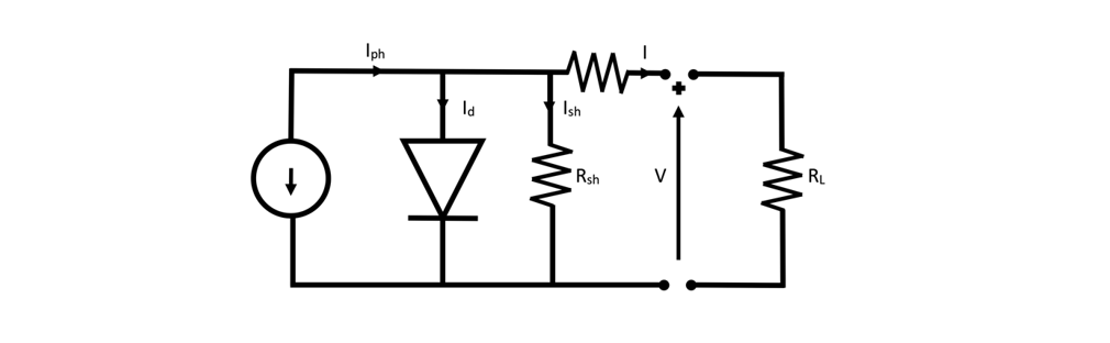
Figure 1 - 1 diode and 5 parameter model
2.1. Initial equations
The electrical current at the output terminals of the photovoltaic cell, I, is mathematically described by equation (1).
(1)
Where Iph represents the electrical current generated in the photovoltaic cell under the presence of light, Id the current that runs through the diode and Ish the current that runs through the resistance Rsh.
The mathematical expression that describes the current that runs through the diode is (2):
(2)
Where V is the electrical voltage at the cell terminals, I0 is the saturation current of the diode, Ns is the number of cells in series of the module and Vt is the thermal potential, given by equation (3).
(3)
Where is the diode ideality factor, kB the Boltzmann constant, T the p-n junction temperature and q the electron charge.
On the other hand, the current flowing through the resistance Rsh is described by equation (4).
(4)
Manipulating equations (1), (2) and (4) [5], it is possible to obtain the equation that describes the I-V characteristics of a photovoltaic cell (5).
(5)
In equation 5 the unknown variables are Iph, I0, Vt, Rs and Rsh. However, these parameters are not provided by the module manufacturer. The objective is to build a model that determines these unknown parameters without any measurement in the system, using only the values provided by the module manufacturer on the datasheet. The following equations will be the five equations needed to determine the five unknowns. Equation (5) can be rewritten for short circuit, maximum power point and open circuit situations, obtaining equations (6), (7) and (8), respectively.
(6)
(7)
(8)
At the point of maximum power, the derivative of power in relation to voltage is zero, that is,
(9)
The derivative of the current in relation to the voltage in the short circuit situation is determined by the resistance Rsh, which is the fifth and last equation needed to determine the five unknowns.
(10)

2.2. Manipulation of initial equations
Through mathematical manipulation [6] it is possible to calculate equations (11), (12) and (13) that allow the determination of the parameters Rs, Rsh and Vt.
(11)
(12)
(13)
Finally, the remaining two unknown variables can be calculated using equations (14) and (15).
(14)
(15)
The data provided in the modules datasheet refer to Standard Test Conditions (STC), that is, with a cell temperature of 25ºC and an irradiance of 1000 W/m2. The determination of the five parameters is made based on the values measured under STC. For the simulation to correctly predict the behavior of the system, it is necessary to take into account the effects of temperature and irradiance.
2.3. Influence of irradiance and temperature on the model
Considering the studied effects, the equations below describe the model parameters, considering simultaneously the effect of temperature and irradiance. The development of these equations can be found in [5] and is supported by [7].
(16)
(17)
(18)
(19)
(20)
2.4. Modeling modules with hotspot
As mentioned above, the resistance Rs represents the resistance to current flow due to the structure of the module, and the losses are due to the Joule effect, where heat is released. Hotspot type defects are regions of the modules that are at a higher temperature compared to the rest of the module.
The model of one diode and five parameters was adapted in order to model a module with hotspot, since the cell containing the hotspot has a higher temperature than the other cells of the photovoltaic module, modifying the model was done by changing the resistance value Rs. Due to the lack of bibliographic information about the modeling of photovoltaic modules with hotspot, the adaptation of the model was made based on experimental data of energy production of the module with this type of defect.
3. Results and experimental model validation
In this study a set of four 327 Wp monocrystalline silicon modules (SunPower, model E20-327), installed in Santarém, Portugal, were used as shown in Figure 2.
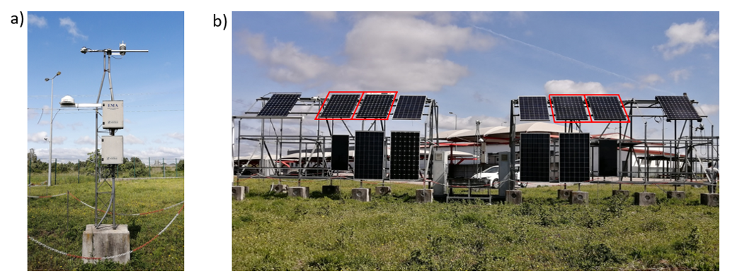
Figure 2 - a) automatic weather station; b) PV modules under study
Voltage and current data were measured for each of the modules as well as meteorological data (irradiance and ambient temperature, among others) over a period of two years. The respective reference thermogram was also registered for each one of the modules (3 of the modules did not have hotspots and one of the modules presented an hotspot of 26.5º C, 12.5 ºC above the same region of the good modules). Figure 3 shows a thermal image of the module with hotspot, a regular photograph and the thermal analysis performed.
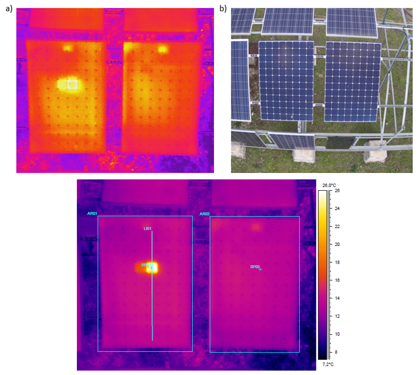
Figure 3 - Thermal image (and photo) of two PV modules (one with hotspot) and its thermal characterization
Starting from the datasheet of the modules and meteorological records (as the only input data) and using the developed model (whose equations can be solved iteratively), the production estimation for each module was determined and adjusted in the case of the module with hotspot. Real production data were used to assess the model's validity.
Since the experimental PV modules are connected to MPPT (Maximum Power Point Trackers) that ensures their operation at the maximum power, it is possible to use the presented model to estimate their power production.
With this experimental work, it was possible not only to validate the model but also to estimate, for the case study, the variation in production due to a hotspot.
Typical results can be found in Figure 4 for a clear sky day and for a cloudy day. The dashed lines stand for real energy production for healthy modules 1, 2 and 3, and real energy production for the module with hotspot; solid lines depict the simulation for both healthy and damaged modules.
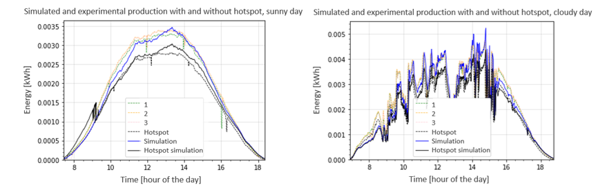
Figure 4 - Experimental typical results for a clear day and for a cloudy one
In the validation of data referring to the healthy module, it was found that the average error between the modeling of the photovoltaic module and the experimental data is always less than 10%. This indicates that the simulation has provides good results for healthy PV modules.
For the module with hotspot, the developed model allowed to obtain results with an error of less than 17.5%. The model presents a worse performance for this type of modules because it is a less consolidated model. However, the model obtained allows us to draw some conclusions:
In 2017 there was a loss of energy production for the module with hotspot of 52.5 kWh, which corresponds to a loss of 10.1%, relative a healthy module.
In 2018, the energy loss was 40.3 kWh, which corresponds to a loss of 8.7%, in relation to the healthy module.
4. Conclusion
This work aimed to evaluate the impact of the presence of a hotspot-type defect, in a photovoltaic module, on energy production. It was concluded that a photovoltaic module with a hotspot-type defect, with temperature difference between the healthy and the defect regions is about 13ºC, can produce 10% less energy than the healthy modules under study. A comparison of the data obtained in the simulation and the experimental data pointed to a difference of 10% for healthy modules and 17.5% for the module with the hotspot, leading to a model validation. Thus, it can be concluded that, with the work developed and the model implemented, with only meteorological data of ambient temperature and global irradiance, as well as the datasheet values of the photovoltaic modules, it was possible to estimate the energy production for a healthy module and for a defective module with a hotspot.
Further work should be developed, using a greater number of modules with defects to extend the experimental data. In this scenario, it would be possible to assess the relation between the severity of each hotspot (in terms of temperature variation) and respective loss of energy production.
With this work, we are developing a decision-aid tool for the management of photovoltaic energy production systems, anticipating possible production losses with thermographic inspections.
References
- H. Glavaš, M. Vukobratović, M. Primorac, and D. Muštran, “Infrared thermography in inspection of photovoltaic panels,” presented at the 2017 International Conference on Smart Systems and Technologies (SST), 2017, pp. 63–68. doi: 10.1109/sst.2017.8188671.
- M. W. Akram et al., “Study of manufacturing and hotspot formation in cut cell and full cell PV modules,” vol. 203, pp. 247–259, Jun. 2020, doi: 10.1016/j.solener.2020.04.052.
- U. Jahn and M. Herz, “Review on Infrared and Electroluminescence Imaging for PV Field Applications,” 2018. Accessed: Dec. 22, 2022. [Online]
- P. Cova, N. Delmonte e M. Lazzaroni, “Photovoltaic plant maintainability optimization and degradation detection: Modelling and characterization”, Microelectronics Reliability, vol. 88-90, pp. 1077–1082, 2018. doi: 10.1016/j.microrel.2018.07 .021. URL: https://doi.org/10.1016/j.microrel.2018.07.021.
- Raimundo, R., 2021, Produção de energia elétrica através de módulos fotovoltaicos com defeitos do tipo hotspot, Master Degree Thesis, Faculdade de Ciências e Tecnologia, Universidade Nova de Lisboa.
- Coelho, A., 2010, New Trends in Photovoltaic Systems - Modeling Power Output With Solar Tracking, Master Degree Thesis, Instituto Superior Técnico, Universidade de Lisboa.
- H. Ibrahim e N. Anani, “Variations of PV module parameters with irradiance and temperature”, Energy Procedia, vol. 134, pp. 276–285, 2017. doi: 10.1016 /j.egypro.2017.09.617