Dynamic performance for interconnection of Inverter Based Resources in weak grids
Authors
D. DHUNGANA, D. RAMASUBRAMANIAN, M. BELLO – Electric Power Research Institute, Palo Alto, California, USA
M. PETERSON - Entergy Services Inc., New Orleans, USA

Summary
This paper presents a methodology and results for efficiently screening weak grid buses in a practical power system with high penetration of inverter-based resource. It also includes time domain analysis results using positive sequence models, focusing primarily on the identified weak buses. The study compares grid behavior using both state-of-the-art positive sequence models available in commercial simulation platforms and the enhanced models initially developed by EPRI, which have since been integrated into commercial simulation platforms. The findings show that relying on a single screening metric is insufficient and multiple metrics are necessary to get a comprehensive understanding of grid strength. Additionally, the paper highlights the need for more accurate and detailed positive sequence models to effectively identify stability issues, especially as grid strength continues to decline globally.
Keywords
AFL, IBR, screening, short-circuit, weak grid1. Introduction
Penetration of Inverter based resources (IBRs) has significantly increased in the recent past, continuing to replace conventional synchronous machine-based resources across most transmission networks. Power systems are expected to be dominated by IBRs in the near future. The vast majority of IBR controls require an interconnection to a strong grid for stable operation. Grid strength at a point of interconnection (POI) bus refers to the grid’s ability to maintain voltage regardless of changes to the current injected at that bus. In other words, grid strength at a POI bus reflects the electrical closeness of that bus to an ideal voltage source. Synchronous machines have traditionally acted as ideal voltage sources behind an impedance. With the decline in synchronous machines and rise in IBRs which, acting in unison, cause large changes in current injected into the grid, grid strength continues to decline in most power systems. This can result in potential stability issues related to IBRs interconnected with weak grid buses. Transmission planners must adequately analyze the performance of these IBRs during interconnection assessments to ensure stable and reliable power system operation. As traditional generators are retired, the resulting reduction in grid strength may no longer support even previously interconnected IBRs. Therefore, the performance of operational IBRs interconnected to the power system must be continually assessed, along with planned future IBRs on the transmission system.
Ideally, the performance of all existing and planned future IBRs would be assessed using detailed Electromagnetic Transient (EMT) based simulations to identify all performance and reliability issues. However, conducting EMT analysis for all IBRs and scenarios is data-intensive, complex and time-consuming, making it largely impractical. Therefore, transmission planners and operators need faster, less sophisticated methods to focus on potential problem areas.
EPRI’s 2018 report, “Guidelines for Studies on Weak Grids with Inverter Based Resources: A Path from Screening Metrics and Positive Sequence Simulations to Point on Wave Simulations” [1], outlines a comprehensive three stage study approach. The first stage involves short circuit based screening of weak grid buses by using steady- state powerflow models only. This is followed by positive sequence dynamic analysis of the identified weak buses using enhanced IBR models that explicitly represent IBR controls. The final stage consists of detailed EMT simulation using appropriate IBR and network models.
EPRI recently conducted a case study on a US based utility system anticipating a significant increase in IBR interconnections in the near future. The study aimed to identify potential instability issues related to IBRs connected to weak grid buses and included all projected IBRs and their interconnection buses for the designated future study year. This case study utilized the first two steps of the three-step process outlined in [1].
In step one, different short circuit based metrics were calculated using steady state powerflow models of the future scenario [2]. Based on this analysis, a subset of IBR connected buses were screened as weak buses. In step two, dynamics analysis of the future scenario was performed using the advanced regc_c model to represent the IBR converter. This paper presents the methodology and selected results from the case study.
2. Powerflow case updates
This study utilizes the US-Canada Eastern Interconnection power system model, with a specific focus on a designated utility footprint. The future scenario includes a large number of planned IBR interconnections at thirty-six different POI buses within the utility’s footprint. Two powerflow cases representing light load and peak load conditions were used for the analysis. The future IBRs were added to the base powerflow cases using a simple modelling approach, as described in [3], which includes an IBR equivalent unit, a padmount transformer, an equivalent collector feeder, and a main power transformer (MPT), as illustrated in Figure 1 below.
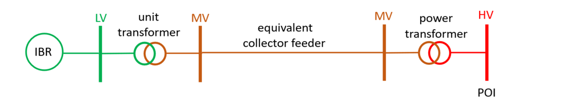
Figure 1 - simple aggregated model for example IBR power plant
Since all IBRs are future units, typical values were used to model their interconnections as below:
- Aggregate IBR Machine: Pmax = maximum IBR MW output, Mbase (MVA) = 1.1 times Pmax, Qmax = ±0.436 times Mbase, voltage control of the POI bus between 1.0 - 1.02 pu (based on pre-existing voltages).
- Equivalent Unit Padmount Transformer: Winding MVA= 1.2 times Mbase, R = 0.005 pu, X=0.06 pu on winding MVA base.
- Equivalent Collector feeder: R = 0.011 pu, X = 0.027 pu, B= 0.069 pu on 100 MVA base. Feeder MVA = Winding MVA
- Main Power Transformer: Winding MVA = 1.2 times Mbase, R = 0.005 pu, X=0.06 pu on winding MVA base
To stress the system, all future IBRs were dispatched at their full rated output (i.e., Pgen = Pmax). To offset the large amount of active power injected by these additional IBRs, an equivalent amount of conventional generation capacity was set offline in the powerflow models. The resulting cases reflected an IBR penetration of up to 32%, as shown in Figure 2 below.
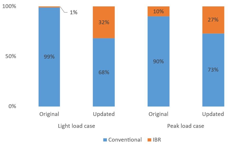
Figure 2 - Conventional Vs IBR generation mix
3. Screening for weak grid
Weak grid buses have traditionally been screened using the short circuit ratio (SCR) metric. At low levels of IBR penetration, SCR offers a convenient way to quickly assess grid strength. While SCR accounts for all synchronous machines and their electrical distances, it does not consider the impact of other IBRs already connected to the system. As IBR penetration continues to grow, this limitation is becoming increasingly significant.
To address this, various metrics have been proposed in the industry, including Available Fault Level (AFL) [4] [5], critical clearing time (CCT) [1], weighed short circuit ratio (WSCR) [6], composite short circuit ratio (CSCR) [7] and short circuit ratio with interaction factors (SCRIF) [4] [8]. Each of these indices has its own advantages, limitations, and specific use cases, which are not discussed in detail in this paper for brevity. Readers are encouraged to review the references for further background on these indices.
An automated tool [2] was used in this study to analyze steady state powerflow cases to evaluate grid strength metrics: SCR, AFL, WSCR, CSCR and CCT under both normal system conditions (no contingency) and contingency scenarios. Metrics were calculated for two system intact powerflow cases, as well as sixteen critical contingencies identified across the thirty-six IBR POI buses. The results from this analysis are discussed in the following sections.
3.1. Short Circuit Ratio (SCR)
As a basic metric, SCR was used in this analysis to identify any obvious weak buses in the system. The range of SCR values calculated is shown in Figure 3. It presents SCR values for the light load and peak load cases under system-intact conditions (i.e., without contingencies), as well as the maximum and minimum SCR values observed across both power flow cases and all studied critical contingencies. To conservatively screen the buses, no short circuit contribution from IBRs was considered, given that IBRs typically produce minimal fault current.
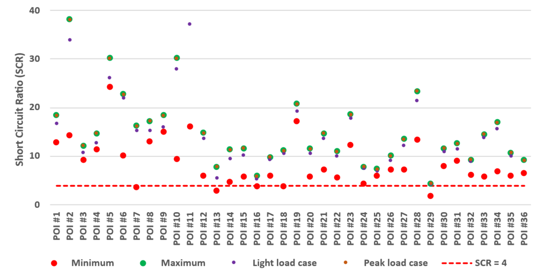
Figure 3 - Short circuit ratio range
It was generally observed that the light load cases exhibit lower SCR values than the peak load cases. This is expected, as the light load case has a higher IBR penetration and fewer synchronous machines online. The lowest SCR values were mostly associated with contingency events in the light load case. Similarly, the highest SCR values were observed exclusively in the peak load case under system-intact conditions, resulting in an overlap between the peak load case and the maximum SCR values, as shown in Figure 3 . Based on the observed SCR range, a threshold of 4 was used to screen for weak buses. Five buses were identified as weak buses based on this criterion, as listed in Table I .
POI Bus | Minimum SCR | Powerflow model |
POI #29 | 1.8 | Light load |
POI #13 | 3.0 | Light load |
POI #7 | 3.7 | Light load |
POI #18 | 3.8 | Light load |
POI #16 | 3.9 | Light load |
3.2. Available Fault Level (AFL)
3.2.1. AFL Background
The AFL metric is based on the concept that IBRs act as sink for short circuit MVA (SCMVA), as outlined in CIGRE Technical Report, “Connection of wind farms to weak AC networks” [4]. The SCMVA at a POI bus is initially calculated using a method similar to that used for determining SCR. The contribution of existing IBRs may or may not be included in this calculation [1].
All IBRs connected to the system are then assumed to draw from the SCMVA at the POI bus, based on an assumed minimum SCR requirement for stable operation. The amount of SCMVA drawn by each IBR depends on its installed capacity, minimum SCR requirement, and electrical distance from the POI bus. That is, IBRs electrically farther from the POI bus draw less SCMVA than those closer, even if they have same installed capacity and minimum SCR requirements.
After deducting the SCMVA drawn by each IBR, the SCMVA balance is defined as the Available Fault Level (AFL) metric. Since this is a theoretical calculation, the AFL can be negative if a large number of IBRs are located near the POI bus. Like other screening metrics, a negative AFL does not mean that no new IBRs can be interconnected at this POI, but it does indicate an elevated risk of stability issues and a heightened need of scrutiny during interconnection assessments.
Evaluation of the AFL metric is illustrated below using an example network shown in Figure 4.

Figure 4 - Example network for AFL metric demonstration
Assume a simple network with two IBRs, each requiring a minimum SCR of 2 for stable operation. Also, assume the total short-circuit MVA at the POI bus has been determined to be 2000 MVA. For this example:
Available SCMVAPOI = 2000 MVA and minSCRIBR1 = minSCRIBR2 = 2
The SCMVA drawn by an IBR from a bus can be calculated with the following equation:
Therefore,
The AFL at POI Bus is then calculated as below:
The calculation of this metric using commercial simulation tools may follow a slightly different implementation approach than illustrated above. For instance, the automated tool [2] used in this study first calculates the SCMVA at the POI bus without considering any IBR contribution. It then recalculates the SCMVA at the same POI bus by assuming that IBRs contribute SCMVA equivalent to min SCR * IBR MVA , achieved by setting IBR source impedance equal to 1/min SCR . The additional SCMVA contributed by IBRs is interpreted as the amount they would draw for stable operation and is therefore subtracted from the SCMVA at the POI bus. Refer to [5] for a demonstration of this approach using a simple example.
The AFL metric is useful for identifying potential weak buses in the system, estimating the required ratings of system strengthening devices, and filtering or ranking buses based on system strength.
3.2.2. Case Study AFL Results
The AFL values evaluated for each POI bus covering both peak and light load cases, as well as the minimum and maximum values across all base cases and contingencies are presented in Figure 5 below.
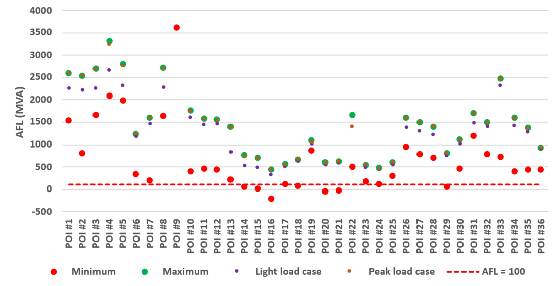
Figure 5 - AFL range
Figure 5 shows that AFL values were generally lower in the light load case compared to the peak load case, consistent with the trend observed for the SCR metric. Based on the distribution of the minimum AFL values, a generic cutoff of 100 MVA was used to identify critical POI buses. The POI buses screened as weak buses based on this threshold are listed in Table II.
Bus Name | Minimum AFL (MVA) | Powerflow model |
POI #16 | -213 | Light load |
POI #20 | -56 | Peak load |
POI #21 | -38 | Peak load |
POI #15 | 5 | Light load |
POI #14 | 50 | Light load |
POI #29 | 57 | Light load |
POI #18 | 80 | Light load |

3.3. Critical Clearing Time (CCT)
The CCT metric is derived from the mathematical analogy between the phased locked loop (PLL) dynamics equation and the conventional swing equation for synchronous machines. It offers an efficient method for identifying potential risks of IBR instability without running full dynamics analysis. However, this CCT metric should not be confused with the conventional critical clearing time associated with angular stability of synchronous machines. Details on the derivation of the CCT metric and its underlying assumptions are provided in [1]. The CCT metric is calculated using the powerflow solution of the pre-fault system and a few controller parameter settings. For this study, the controller parameters were based on generic assumptions, as shown in Table III.
Parameter | Value | |
| PLL gains | Proportional | 60 |
Integral | 200 | |
| Outer voltage control loop gains | Proportional | 40 |
Integral | 1 | |
| IBR maximum current | 1.1 | |
| IBR maximum reactive current | 1 | |
| Voltage measurement transducer time constant (sec) | 0.02 | |
| Breaker and relay time (second) | 0.1 | |
| PQ priority flag | Q priority | |
The CCT values evaluated for each POI bus covering both peak and light load cases, as well as the minimum and maximum values across all base cases and contingencies are presented in Figure 6.
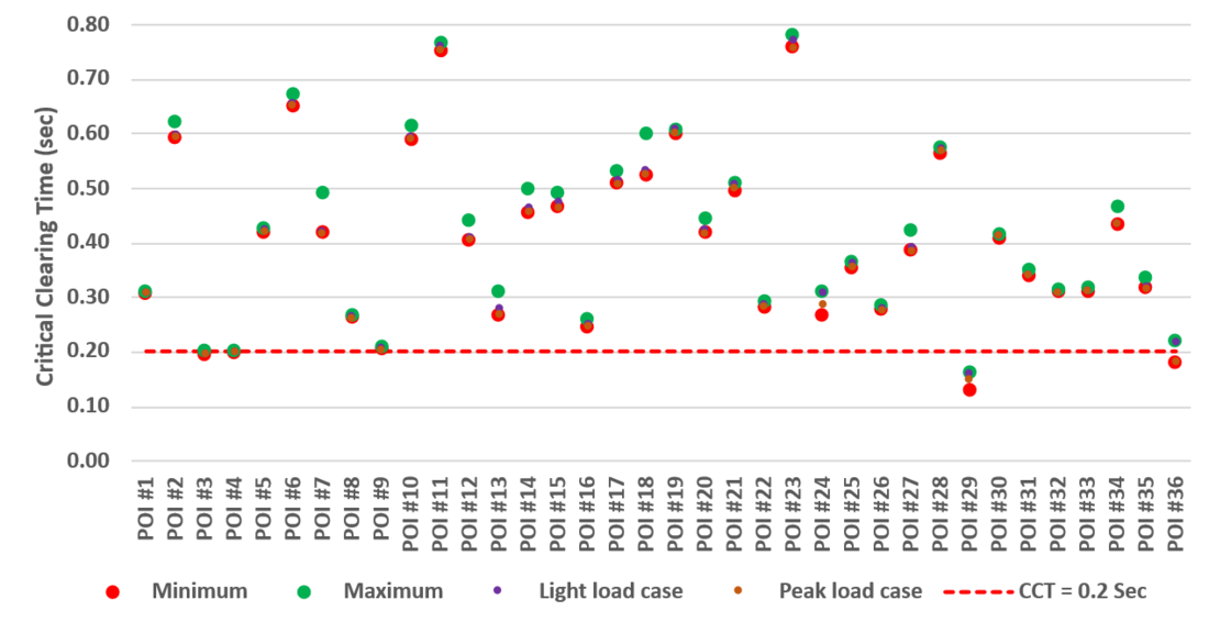
Figure 6 - CCT range
CCT metric is influenced by the grid strength at the IBR terminal bus, as well as the active and reactive power outputs from the IBR [1]. Since the active power output from the IBRs was set to their maximum across both cases and contingencies, with some variation in reactive power outputs and minor changes in grid strength, the resulting CCT values showed minimal variation. Based on the observed results, a threshold of 0.2 seconds was used to screen critical POI buses. The POI buses identified using this threshold are listed in Table IV. Notably, two new POI buses (POI #36 and #3) were identified through this analysis that were not flagged by the previous screening methods.
Bus Name | Minimum CCT (Sec) | Powerflow model |
POI #29 | 0.132 | Light load |
POI #36 | 0.182 | Peak load |
POI #3 | 0.197 | Peak load |
3.4. Weighed and Composite Short Circuit Ratio (WSCR and CSCR)
In scenarios where IBRs are clustered in specific areas of the grid, the WSCR and CSCR metrics can be used to calculate the combined short circuit ratios for those clusters. However, in this case study, the utility did not identify any distinct IBR clusters. Additional analysis using perturbation methods with varying voltage deviation thresholds also yielded inconclusive results. As a result, WSCR and CSCR were not used for screening in this study.
3.5. Identified weak buses
Based on the analysis presented in this section, the screened weak buses are summarized in Table V.
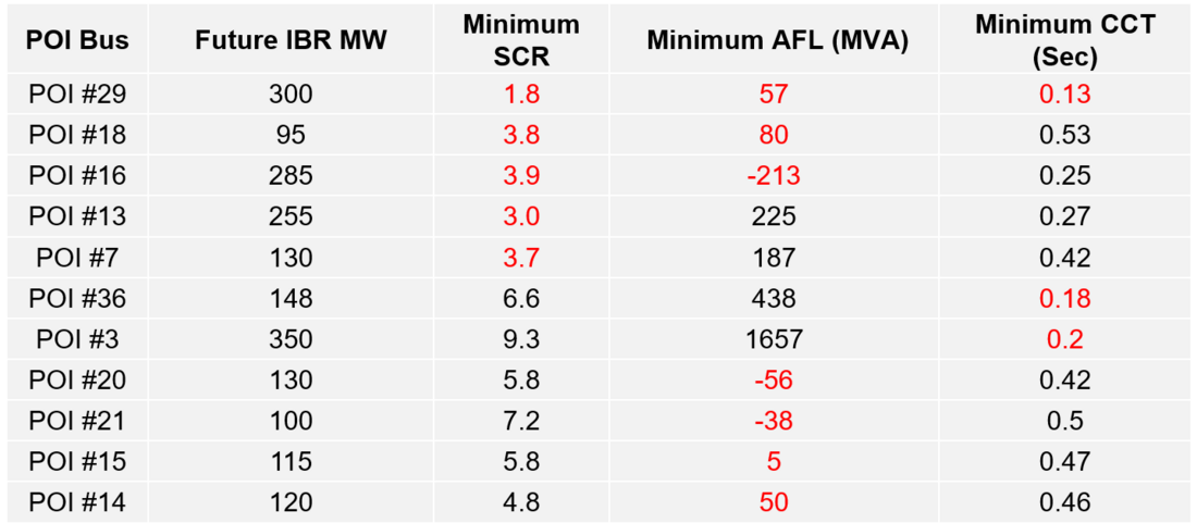
Table V - Identified weak buses
Table V demonstrates that the three metrics used in this study do not consistently identify the same buses as “weak,” but they are directionally aligned. Since the screening is based on limited modeling information and a simplified methodology designed to cover a large number of network buses, no single metric can provide a complete picture of system weak points. Therefore, it is recommended to use multiple complementary screening metrics to rank potentially weak buses.
4. Positive sequence stability analysis
4.1. Methodology
Positive sequence stability analysis was conducted on the utility system, focusing on the weak buses identified in Table V. The methodology used for this analysis is illustrated in Figure 7 .
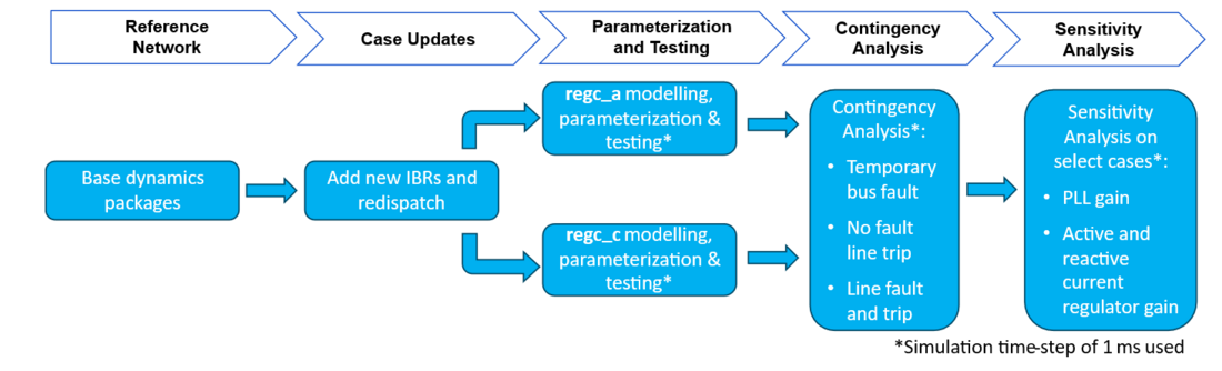
Figure 7 - Positive sequence dynamics analysis methodology
4.2. Model Parameterization and Testing
The dynamics package, which included both power flow and dynamic models, was used as the starting point for this analysis. As discussed in Section 2, future IBRs were added to the original powerflow models and dispatched at full output, requiring the removal of an equivalent amount of conventional generation capacity. Two sets of dynamic models for the future IBRs were developed, using the state-of-the-art regc_a model [3] and the newer regc_c model [9] [3] to represent the generator/converter. The model parameters used for both regc_a and regc_c are provided in Appendix A. Since the regc_a and regc_c converter models have distinct parameter sets, most of which cannot be directly mapped, generic parameters were selected for each model.
In both model sets, the electrical and plant controls were represented using the reec_a and repc_a models with typical parameters, as listed in Appendix A. The updated dynamic model packages for the two sets demonstrated acceptable flat-run responses (i.e., no disturbance applied), as shown by the terminal voltage plots across future IBRs connected to weak buses in Figure 8.
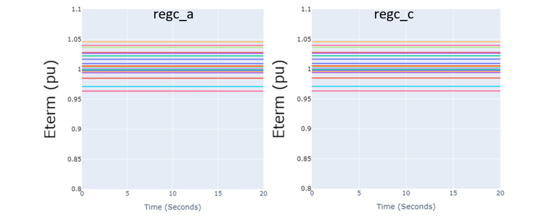
Figure 8 - Future IBRs (connected to weak buses) terminal voltages during flat run
4.3. Contingency Analysis
4.3.1.Temporary bus fault
Three-phase temporary bus faults with a typical 6-cycle fault duration were applied at each of the weak POI buses for this analysis. This type of contingency was chosen because temporary faults without topology changes can sometimes elicit interesting converter model responses. As shown in Table V, POI #3 has a future IBR interconnection of 350 MW, the largest among the future IBRs connected to weak buses. The terminal voltage responses of the IBR at POI #3 for all analyzed contingencies are presented in Figure 9.
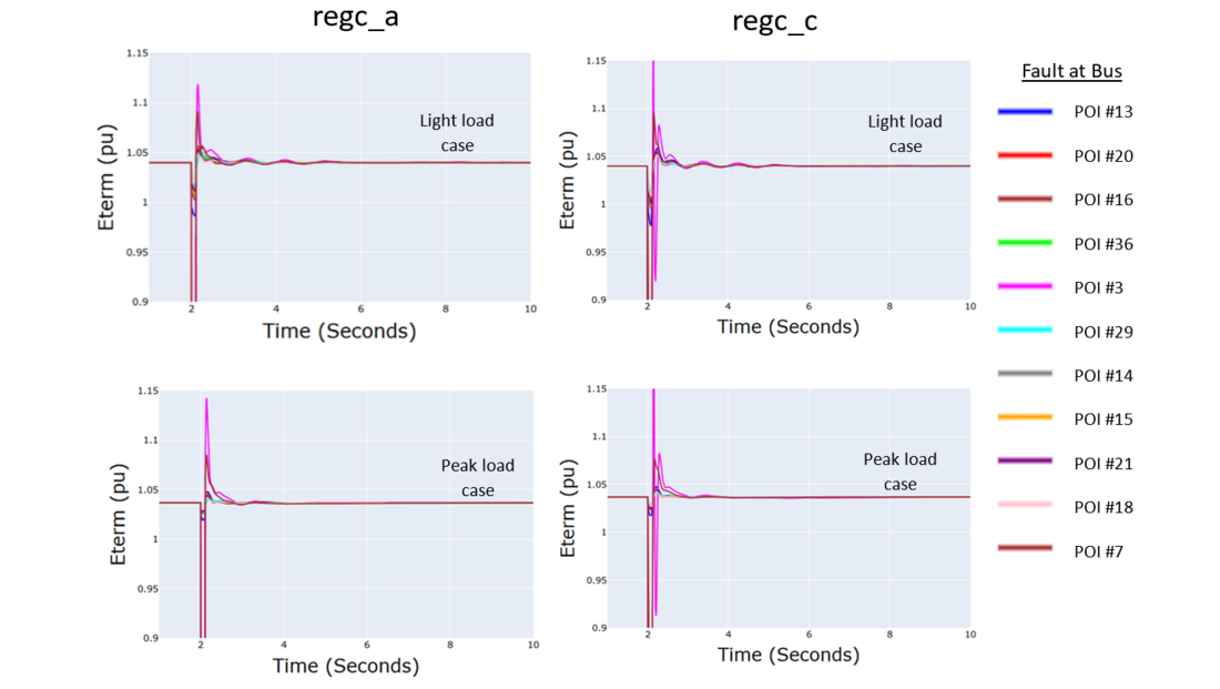
Figure 9 - Terminal voltages of IBR at POI #3 for ‘temporary bus fault’ contingencies
Figure 9 shows that neither model exhibits undamped oscillations, and their responses are comparable. The state-of-the-art regc_a is a current-source interface model, while regc_c is a voltage-source interface model that includes an inner current control loop and a phase-locked loop (PLL) [3] [10] [11] [12]. In weak grid applications, regc_a experienced numerical stability issues, leading to non-convergence during close-in faults. This behavior is illustrated in Figure 10, which presents network convergence across various scenarios for both models.
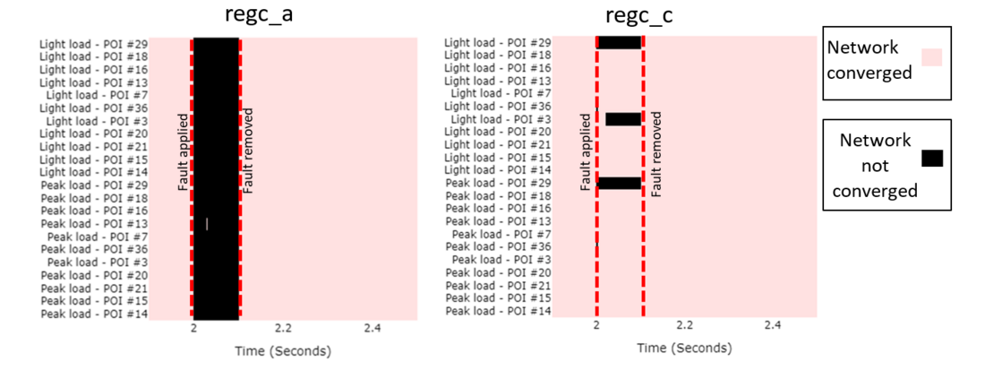
Figure 10 - Network convergence for ‘temporary bus fault’ at weak buses
4.3.2. No fault line trip
This type of disturbance was studied because no-fault disturbances typically produce minimal responses from electrical and plant control models, making it easier to analyze generator/converter model behavior. For this analysis, contingencies involving a single line trip without fault were assessed at each of the weak buses. Figure 11 presents the fifteen terminal voltage channels that exhibited the largest oscillation magnitudes among all future IBRs connected to weak buses across the assessed contingencies.
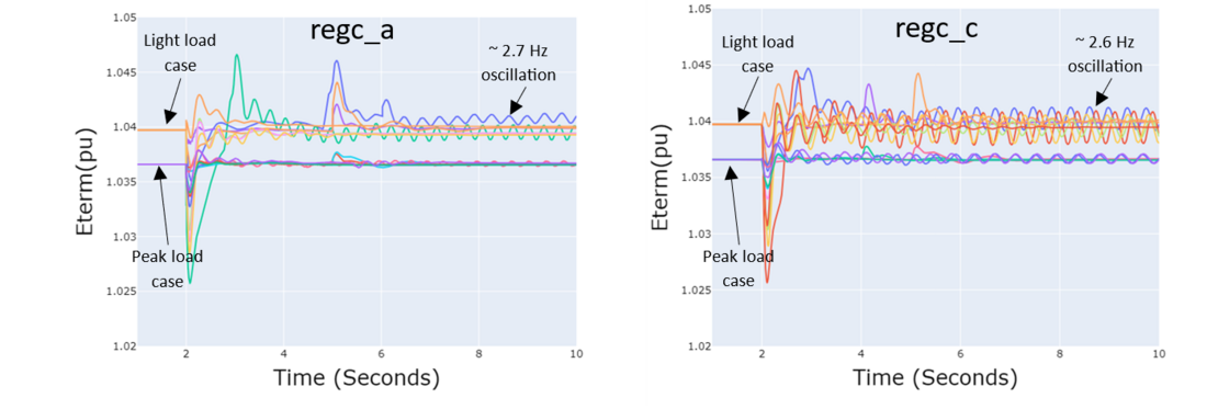
Figure 11 - Future IBR terminal voltage outputs for ‘no fault line trip’ contingencies
In the first plot, some IBR generators modeled with the regc_a model exhibited undamped oscillations. In the second plot, which shows results for IBR generators modeled with the regc_c model, these oscillations increased in magnitude, and several additional IBR generators displayed undamped oscillations. The increased oscillations in the second plot can be attributed to the use of the regc_c converter model.
4.3.3. Line fault and trip
Line faults and line trips are typical N-1 contingencies studied by Transmission Planners for compliance purposes. This analysis included contingencies involving a single line terminated at each of the weak buses, as well as critical contingencies identified by the utility. A three-phase fault at one of the line terminals, lasting for a 6-cycle duration and followed by a line trip, was simulated. The fault duration of 6 cycles is half the critical clearing time (CCT) threshold used to screen weak buses, as described in Section 3.3. Figure 12 presents the fifteen terminal voltage channels that exhibited the largest oscillation magnitudes among all future IBRs connected to weak buses across the assessed contingencies.
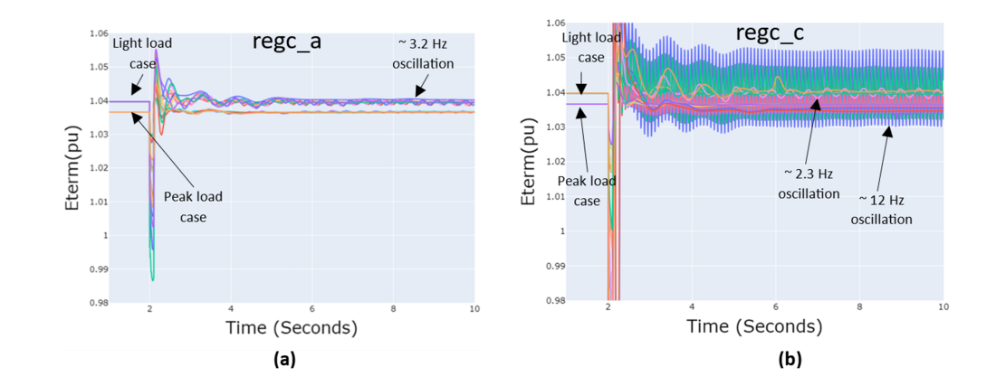
Figure 12 - Future IBR terminal voltage outputs for ‘line fault and trip’ contingencies
As shown above, the responses using regc_a models in Figure 12 (a) exhibit a few low-magnitude undamped oscillations. In contrast, the responses using regc_c models in Figure 12 (b) show a greater number of IBRs with undamped oscillations, some occurring at relatively higher frequencies. Certain curves in Figure 12 (b) display oscillations reaching up to 12 Hz, which approaches the bandwidth limit of positive sequence simulation tools. The presence of such high-frequency oscillations suggests that detailed EMT studies may be necessary. Regardless, the presence of sustained oscillations in the output warrants further investigation, most likely through detailed EMT studies.
Consistent with the observations from Figure 10, the regc_a model leads to network non-convergence in a larger number of fault scenarios near the IBRs compared to the regc_c model. However, a plot illustrating this behavior is not included in this paper for brevity.
4.4. Detailed Example and Sensitivity Analysis
Section 4.3 highlights the general trends in the differences observed when using either of the generator/converter models. This section presents a detailed example of those differences, along with a sensitivity analysis of the regc_c gain parameters. Figure 13 shows the terminal voltage response for the 285 MW IBR interconnected at POI #16 during a generator unit trip contingency, which does not involve any fault. The generator that was simulated to trip is a 100 MW unit located approximately 25 miles away.
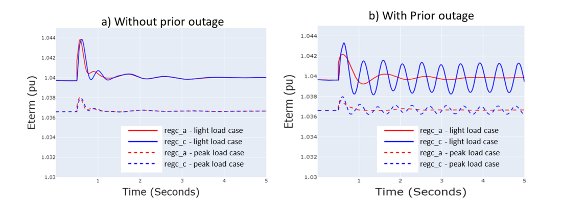
Figure 13 - IBR at POI #16 terminal voltage for a specific unit trip contingency
Figure 13 presents plots for scenarios with and without a prior outage of a nearby line, which generally reduces system strength at the POI bus. System strength metrics for the two analyzed power flow cases are shown in Table VI. The table indicates a significant reduction in the AFL metric, a slight reduction in the SCR metric, and a very small increase in the CCT metric. The slight increase in the CCT metric in the prior outage cases is attributed to a reduction in MVAR output from the unit, caused by topology changes resulting from the outage. This reduction influenced the metric more than the decrease in equivalent impedance.
Figure 13(b) shows undamped oscillations for the IBR at POI #16 under reduced system strength conditions caused by a prior outage of a transmission line. This example demonstrates that the state-of-the-art regc_a model may not be adequately capture IBR dynamics in weak grid conditions, potentially leading to false positive results. Although the SCR and CCT metrics do not change significantly in this scenario, the AFL metric shows a substantial decrease. This suggests that these metrics should be used in a complementary manner.
Metric | Light load case | Peak load case | ||
Without prior outage | With prior outage | Without prior outage | With prior outage | |
| SCR | 5.36 | 4.12 | 5.80 | 4.25 |
| AFL (MVA) | 26 | -426 | 175 | -413 |
| CCT (sec) | 0.576 | 0.588 | 0.556 | 0.559 |
For the oscillatory response observed in Figure 13(b), a sensitivity analysis was performed by varying the gain parameters in the regc_c model. The gain variations are detailed in Table VII. Figure 14 shows the terminal voltage response of the IBR at POI #16 under light load conditions with a prior outage, for different regc_c model gain settings.
Parameter | Default | High | Low |
| Proportional gain on PLL regulator (KPPLL) | 60 | 120 | 30 |
| Integral gain on PLL regulator (KIPLL) | 1400 | 2800 | 700 |
| Proportional gain on reactive current regulator (KPQ) | 1 | 2 | 0.5 |
| Integral gain on reactive current regulator (KIQ) | 50 | 100 | 25 |
| Proportional gain on active current regulator (KPP) | 1 | 2 | 0.5 |
| Integral gain on active current regulator (KIP) | 50 | 100 | 25 |
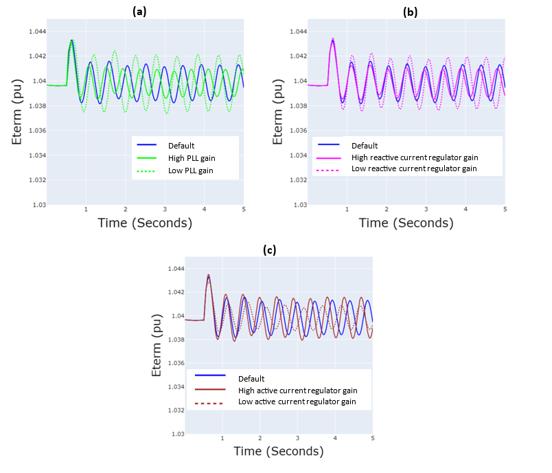
Figure 14 - Sensitivity of regc_c response on gain parameters
Sensitivity analysis results presented in Figure 14(a) and Figure 14(b) indicate that increasing the gains of the phase-locked loop (PLL) and reactive current regulator leads to a reduction in oscillation magnitude. Figure 14(c) shows that decreasing the active current regulator gain also reduces the oscillation magnitude. These findings are consistent with other examples, which are not included in this paper. This result provides an important insight: gain parameters in the regc_c model may be tuned to enhance stability performance of IBRs under weak grid conditions.
5. Conclusion
Short-circuit-based metrics derived from power flow models were used in this study to efficiently screen for weak grid buses in a utility’s future system with high IBR penetration. The SCR, AFL, and CCT metrics were applied to identify a diverse set of weak buses, each from a slightly different analytical perspective. Positive-sequence dynamic analysis was then performed on the utility’s future system using both the state-of-the-art regc_a model and the newer regc_c model to represent future IBR converters, with a focus on the screened weak buses.
This analysis demonstrated that while the regc_a model is sufficient for representing dynamics in strong grid conditions, it is not adequate for weak grid scenarios. The regc_c model, which includes a more detailed representation of inner control loops, is better suited for modeling IBR converters connected to weak grids. However, further EMT-based analysis of the utility’s future system is necessary to validate the accuracy of the responses produced by the regc_c model in comparison to those from the regc_a model. This validation could not be conducted within the current study due to constraints in project scope and available funding.
References
- EPRI, "Guidelines for Studies on Weak Grids with Inverter Based Resources: A Path from Screening Metrics and Positive Sequence Simulations to Point on Wave Simulations. EPRI, Palo Alto, CA: 2018. 3002013639."
- "PRE-SW: Grid Strength Assessment Tool (GSAT) Version 6.0 Beta. EPRI, Palo Alto, CA., 3002027116," 2023. [Online].
- "Model User Guide for Generic Renewable Energy System Models: EPRI, Palo Alto, CA: 2023. 3002027129.".
- CIGRE WG B4.62, "TB 671: Connection of Wind Farms to Weak AC Networks," CIGRE, 2016.
- D. Ramasubramanian, "Location and Sizing of Grid Forming Devices in Transmission Power Networks," in C4 Power System Technical Performance, PS1 Power system dynamic analysis in the energy transition: challenges, opportunities and advances, Paris, 2024 - Ref C4-10456-2024.
- Y. Zhang, S.-H. F. Huang, J. Schmall, J. Conto, J. Billo and E. Rehman, ""Evaluating system strength for large-scale wind plant integration," in 2014 IEEE PES General Meeting, National Harbor, MD, 2014.
- R. Fernandes, S. Achilles and J. MacDowell, "Report to NERC ERSTF for composite short circuit ratio (CSCR) estimation guideline," GE Energy Consulting, 2015.
- NERC, "Integrating Inverter-Based Resources into Low Short Circuit Strength Systems, Reliability Guideline," 2017. [Online]
- D. Ramasubramanian, W. Wang, P. Pourbeik, E. Farantatos, A. Gaikwad, S. Soni and V. Chadliev, "Positive sequence voltage source convertermathematical model for use in low shortcircuit systems," IET Generation, Transmission & Distribution, vol. 14, pp. 87-97, 2019.
- J. Hu, Q. Hu, B. Wang, H. Tang and Y. Chi, "Small Signal Instability of PLL-Synchronized Type-4 Wind Turbines Connected to High-Impedance AC Grid During LVRT," IEEE Transactions on Energy Conversion, vol. 31, no. 4, pp. 1676-1687, 2016.
- J. Z. Zhou, H. Ding, S. Fan, Y. Zhang and A. M. Gole, "Impact of Short-Circuit Ratio and Phase-Locked-Loop Parameters on the Small-Signal Behavior of a VSC-HVDC Converter".
- D. Ramasubramanian, X. Wang, S. Goyal, M. Dewadasa, Y. Li, R. J. O'Keefe and P. F. Mayer, "Parameterization of generic positive sequence models to represent behavior of inverter based resources in low short circuit scenarios," Electric Power Systems Research, vol. 213, 2022.
Appendix – Positive Sequence Model Parameters
Value | Description |
1 | Lvplsw (Low Voltage Power Logic) switch (0: LVPL not present, 1: LVPL present) |
0.02 | Tg, Converter time constant, second |
10 | Rrpwr, LVPL ramp rate limit (pu/s) |
0.75 | Brkpt, LVPL voltage 2 (pu) |
0 | Zerox, LVPL voltage 1 (pu) |
0.23 | Lvpl1, LVPL gail (pu) |
2 | Volim, Voltage limit for High Voltage Reactive Current Management, pu |
0.1 | Lvpnt1, High Voltage point for Low Voltage Active Current Management, pu |
0.05 | Lvpnt0, Low Voltage point for Low Voltage Active Current Management, pu |
-0.4357 | Iolim, Current limit for HVRCM, pu (< 0) |
0.02 | Tfltr, Voltage filter time constant for LVRCM (s) |
0 | Khv, Overvoltage compensation gain used in HVRCM (>=0 and < 1) |
10 | Iqrmax, Upper limit on Rate of change for reactive current (pu/s) |
-10 | Iqrmin, Lower limit on Rate of change for reactive current (pu/s) |
0.1 | Accel, Acc. factor for smoothing out voltage & angle calculations (>0 and <=1) |
Value | Description |
0 | PQflag –current priority flag (1=Ip priority, 0=Iq priority) |
1 | PLLFLG –Enables/Disables PLL (1=enabled, 0=disabled) |
1 | KPQ–Proportional gain on reactive current regulator |
50 | KIQ–Integral gain on reactive current regulator |
1 | KPP–Proportional gain on active current regulator |
50 | KIP–Integral gain on active current regulator |
0.0083 | TE–Current delay time constant |
60 | KPPLL–Proportional gain on PLL regulator |
1400 | KIPLL–Integral gain on PLL regulator |
75.4 | Dwmax–Maximum angular speed limit |
-75.4 | Dwmin–Minimum angular speed limit |
10 | rrcur –Maximum rate of change of active current command |
1.1 | Imax –maximum current limit (pu) |
Value | Description |
|---|---|
0 | Input this as 0. For remote bus control use the plant controller model |
0 | PFFLAG (Power factor flag): 1 - power factor control; 0: Q control |
0 | VFLAG: 1 if Q control; 0 voltage control |
0 | QFLAG: 1 if voltage/Q control; 0 if pf/Q control |
0 | PFLAG: 1 If Ipcmd is speed dependent, else 0 |
0 | PQFLAG: 1 for P priority, 0 for Q priority |
0.8 | Vdip (pu), low voltage threshold for reactive current injection |
1.5 | Vup (pu), high voltage threshold for reactive current injection |
0.02 | Trv (s), Voltage filter time constant |
-0.1 | dbd1 (pu), Voltage error dead band lower threshold (<=0) |
0.1 | dbd2 (pu), Voltage error dead band upper threshold (>=0) |
0 | Kqv (pu), Reactive current injection gain |
0.4357 | Iqhl (pu), Upper limit on reactive current injection Iqinj |
-0.4357 | Iqll (pu), Lower limit on reactive current injection Iqinj |
1 | Vref0 (pu), User defined reference (if 0, initialized by model) |
0 | Iqfrz (pu), Value at which Iqinj is held following voltage dip |
0 | Thld (s), Time that Iqinj is held at Iqfrz following voltage dip |
0 | Thld2 (s) (>=0), Time for which IPMAX is held at faulted value |
0.05 | Tp (s), Filter time constant for electrical power |
0.4357 | QMax (pu), limit for reactive power regulator |
-0.4357 | QMin (pu) limit for reactive power regulator |
1.1 | VMAX (pu), Max. limit for voltage control |
0.9 | VMIN (pu), Min. limit for voltage control |
0 | Kqp (pu), Reactive power regulator proportional gain |
0 | Kqi (pu), Reactive power regulator integral gain |
0 | Kvp (pu), Voltage regulator proportional gain |
0 | Kvi (pu), Voltage regulator integral gain |
0 | Vbias (pu), User-defined bias (normally 0) |
0.02 | Tiq (s), Time constant on delay s4 |
2 | dPmax (pu/s) (>0) Power reference max. ramprate |
-2 | dPmin (pu/s) (<0) Power reference min. ramprate |
1 | PMAX (pu), Max. power limit |
0 | PMIN (pu), Min. power limit |
1 | Imax (pu), Maximum allowable total converter current limit |
0.02 | Tpord (s), Power filter time constant |
0 | Vq1 (pu), Reactive Power V-I pair, voltage |
1 | Iq1 (pu), Reactive Power V-I pair, current |
2 | Vq2 (pu) (Vq2>Vq1), Reactive Power V-I pair, voltage |
1 | Iq2 (pu) (Iq2>=Iq1), Reactive Power V-I pair, current |
0 | Vq3 (pu) (Vq3>Vq2), Reactive Power V-I pair, voltage |
0 | Iq3 (pu) (Iq3>=Iq2), Reactive Power V-I pair, current |
0 | Vq4 (pu) (Vq4>Vq3), Reactive Power V-I pair, voltage |
0 | Iq4 (pu) (Iq4>=Iq3), Reactive Power V-I pair, current |
0 | Vp1 (pu), Real Power V-I pair, voltage |
1 | Ip1 (pu), Real Power V-I pair, current |
2 | Vp2 (pu) (Vp2>Vp1), Real Power V-I pair, voltage |
1 | Ip2 (pu) (Ip2>=Ip1), Real Power V-I pair, current |
0 | Vp3 (pu) (Vp3>Vp2), Real Power V-I pair, voltage |
0 | Ip3 (pu) (Ip3>=Ip2), Real Power V-I pair, current |
0 | Vp4 (pu) (Vp4>Vp3), Real Power V-I pair, voltage |
0 | Ip4 (pu) (Ip4>=Ip3), Real Power V-I pair, current |
Value | Description |
|---|---|
Remote bus number or 0 for local voltage control | |
0 | Monitored branch FROM bus |
0 | Monitored branch TO bus |
'0' | Monitored branch ID (enter within single quotes) |
0 | VCFlag, droop flag (0: with droop,1: line drop compensation) |
1 | RefFlag, flag for V or Q control(0: Q control, 1: V control) |
1 | Fflag, 0: disable frequency control, 1: enable |
0.02 | Tfltr, Voltage or reactive power measurement filter time constant (s) |
0.1 | Kp, Reactive power PI control proportional gain (pu) |
0.1 | Ki, Reactive power PI control integral gain (pu) |
0 | Tft, Lead time constant (s) |
0.1 | Tfv, Lag time constant (s) |
0.8 | Vfrz, Voltage below which State s2 is frozen (pu) |
0 | Rc, Line drop compensation resistance (pu) |
0 | Xc, Line drop compensation reactance (pu) |
0.1314 | Kc, Reactive current compensation gain (pu) |
1 | emax, upper limit on deadband output (pu) |
-1 | emin, lower limit on deadband output (pu) |
-0.001 | dbd1, lower threshold for reactive power control deadband (<=0) |
0.001 | dbd2, upper threshold for reactive power control deadband (>=0) |
0.4357 | Qmax, Upper limit on output of V/Q control (pu) |
-0.4357 | Qmin, Lower limit on output of V/Q control (pu) |
1 | Kpg, Proportional gain for power control (pu) |
1 | Kig, Integral gain for power control (pu) |
0.02 | Tp, Real power measurement filter time constant (s) |
-0.0006 | fdbd1, Deadband for frequency control, lower threshold (<=0) |
0.0006 | fdbd2, Deadband for frequency control, upper threshold (>=0) |
999 | femax, frequency error upper limit (pu) |
-999 | femin, frequency error lower limit (pu) |
1 | Pmax, upper limit on power reference (pu) |
0 | Pmin, lower limit on power reference (pu) |
0.02 | Tg, Power Controller lag time constant (s) |
20 | Ddn, droop for over-frequency conditions (pu) |
20 | Dup, droop for under-frequency conditions (pu) |
- [1] IBR contribution to SCMVA were not included in this case study, resulting in more conservative AFL values