Deep Learning for High-Resolution 3D Pressure Fields and Fluid-Flow Distribution in OD/KD Transformer Windings
Authors
G. FLECK - Siemens Energy, Austria
T. KRONLACHNER, R. SONNLEITNER, P.M. BLIES - Emmi AI, Austria
N. GAVRILOV, G. LEVAK - Končar Power Transformers, Croatia
V. ATHREYA - Siemens Energy, Germany

Summary
The methodology for designing large power transformers has become increasingly rigorous, particularly regarding verification. For pump-driven liquid forced and directed cooled transformer configurations, accurate specification of fluid flow distribution between windings and compartments is critical. While 3D Computational Fluid Dynamics (CFD) has been established as the standard for verifying hydraulic properties, the computational cost remains a significant barrier. Despite advancements in processing power, these simulations can take hours or even days. This prohibitive runtime restricts the use of high-fidelity 3D CFD in the early design stages, where its application would otherwise provide invaluable guidance.
Instead, in current industrial practice, the preliminary design stage relies heavily on hydraulic network models to estimate how fluid flows through the transformer. These methods operate by translating the complex, real-world geometry of the components into a system of interconnected nodes and branches. Because this approach simplifies physical details, it forces engineers to rely on empirical assumptions to calculate flow and pressure. While these network models are generally robust enough for standard designs, they fundamentally lack the high level of detail provided by 3D CFD simulations. Consequently, they often fail to capture the full flow behavior emerging from the 3D nature of the geometry in question, which cannot be reduced to a 2D or network model without modelling error. This becomes critical when designing more complex winding arrangements.
To address this gap, we train a machine learning-based surrogate model that approximates the CFD simulation with high fidelity while minimizing computational cost. This enables rapid prototyping based on high-quality results already in early design stages.
The surrogate model can estimate the pressure drop for a defined oil flow in near real-time, achieving a speedup of four orders of magnitude for global pressure drop calculation and a speedup of about 300x for the full 3D reconstruction compared to conventional 3D CFD simulations. This efficiency enables the generation of high-fidelity flow characteristic curves much faster than is possible with CFD, which then only serves the purpose of verifying discrete points on the curve to guarantee final accuracy.
The application of this methodology currently focuses on Zig-Zag windings and axial channel cooled windings. These geometries present unique hydraulic challenges that make them ideal candidates for initial validation. Although this study is restricted to these configurations, the underlying framework is designed for scalability, and future work will extend its application to more complex winding topologies.
Keywords
Transformer, directed cooling, fluid distribution, machine learning, surrogate model1. Introduction
In this work, we describe the creation of a machine learning based surrogate model for hydraulics in the context of large power transformers. In this section, we first describe the cooling types and fluid flow distribution between windings. Later, we introduce the two specific common winding types that we will focus on in this work, the so-called “Zig-Zag cooled” and “axial channel cooled” windings. These sections set the stage to introduce the machine learning surrogate modelling approach. Finally, we show results in the form of qualitative and quantitative validation and conclude our findings.
1.1. Cooling types of transformers
Large power transformers primarily utilize insulating liquids for thermal management. These liquids must exhibit high dielectric strength, superior impregnation capabilities, and excellent thermal properties while ensuring oxidation resistance and material compatibility [1]. In industrial cooling nomenclature, the first letter designates the liquid type: 'O' represents mineral oil, while 'K' refers to 'K-class' insulating fluids - those with a fire point exceeding 300 °C.
The coolant circulates between the heat-generating components and the cooling equipment. This flow is driven either by natural convection (ON/KN) or forced flow via pumps (OF/OD/KF/KD). Forced flow is further distinguished by whether the fluid is directed solely through the external cooling equipment (OF/KF) or forced specifically through the main windings (OD/KD) [2,3,4].
OD and KD configurations are essential for high-capacity transformers. By channeling fluid through defined paths, these systems effectively mitigate hot spots within the windings. Furthermore, directed flow allows for higher power density and optimized material usage, which are critical for meeting the strict spatial constraints and compact design requirements of modern power grids.
1.2. Fluid flow distribution between windings in OD/KD transformers
A transformer has several windings, therefore proper design balances the coolant flow through the windings to control winding temperatures. An example with two windings is visualized in Figure 1 using the flow-pressure characteristics of the individual windings and the resulting total system. In OD/KD‑cooled transformer windings, the longitudinal fluid temperature rise along the winding height - from bottom to top - is typically on the order of 10 K. Since the temperature change of the coolant through the winding is small, it can be assumed that the viscosity and density of the coolant is constant. Therefore, calculation of the pressure drop characteristic with constant fluid properties as a function of fluid flow is a good estimation for OD/KD windings in their typical operating range.
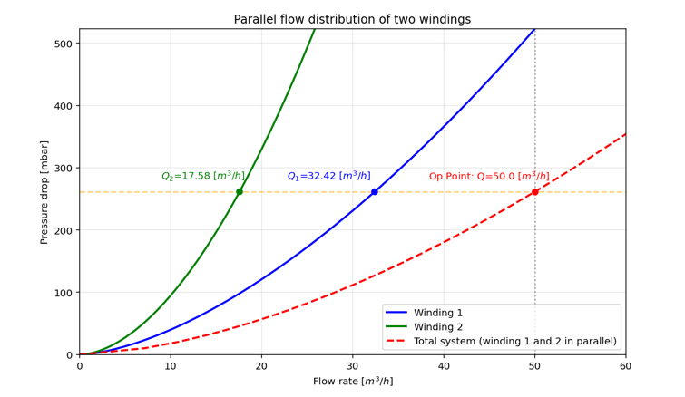
Figure 1 – Example of the parallel flow distribution in two windings for a given oil flow
2. Cooling inside windings
In the previous chapter, the overall cooling types were discussed. Here, we have a closer look at the inner structure of the windings. There is a wide variety of cooling types inside the winding. Main elements to create cooling ducts are spacers, sticks, clack bands and fluid barriers. For this investigation, we focus on two common OD/KD cooled winding types.
2.1. Zig-Zag cooled windings
The Zig-Zag channel cooled winding is a common type for OD/KD cooled transformers, which is investigated in several studies [5,6,7,8]. Specific to this winding type is a guided flow where the vertical channels are blocked in an interleaved manner on the inside and the outside, resulting in a flow in the radial channels alternating from the inside to the outside and vice versa.
Figure 2 shows a 2D schematic slice of the winding visualizing the flow direction in the individual channels (left) and the corresponding simplified network model graph [6,7] (right).
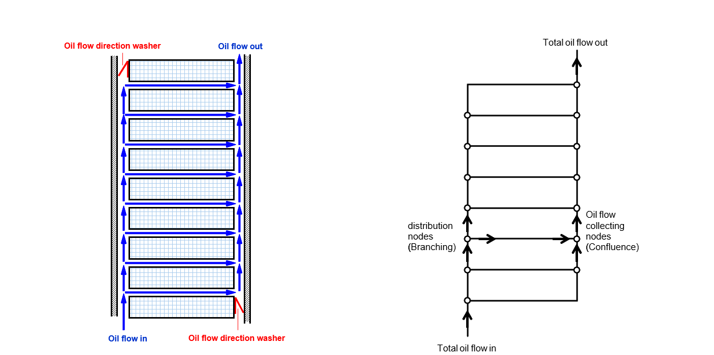
Figure 2 – Schematic of a Zig-Zag cooled winding on the left and the network model abstraction on the right. The figure on the left depicts a cross-section of the winding with the inner axial channel on its left side and the outer axial channel on the right side, respectively
2.2. Axial Channel Cooled Winding
The axial channel cooled winding is a specialized design used primarily in large power transformers. Unlike traditional radial cooling where oil flows horizontally across the discs, this design prioritizes vertical oil flow through the winding. These vertical channels are created by clack bands, which are applied with the conductors during the manufacturing process. The clacks represent obstacles for the fluid flow and create complex flow patterns. Figure 3 shows a 2D schematic slice of the winding visualizing the flow direction in the individual channels. Additionally, the simplified network model graph [6,7] is shown.
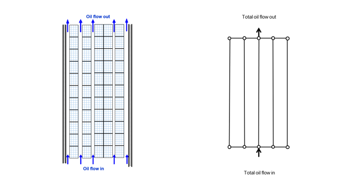
Figure 3 - Schematic of an axial channel cooled winding on the left and the network model abstraction on the right. The widths of the three central axial channels in the left figure are determined by the individual clack bands.
3. 3D CFD modelling of Large Power Transformer Windings
Simulating the full 3D geometry of such a winding design would be redundant because the winding can be decomposed into equal sectors. This allows a reduction of computational effort needed by only calculating one sector. These sectors are defined as the region between two vertical spacers around the circumference. Although it can be assumed that the flow is similar in each of these sections, minor differences can occur, e.g. due to conductor transpositions, non-complete turns, conductor entry, and exits. Figure 4 shows a Zig-Zag winding and the corresponding sector removed. The boundary conditions used in the simulation are inlet flow rate and a constant pressure of zero at the outlet.
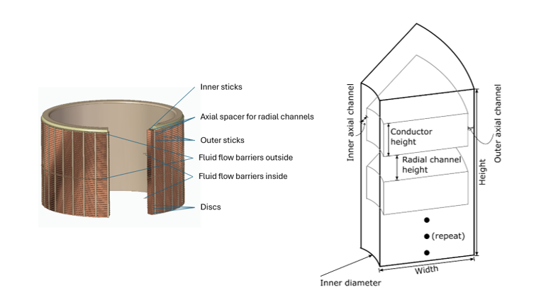
Figure 4 - Sketch of a Zig-Zag-Winding with of sector cut out and the basic dimensions
3.1. Incompressible flow formulation
In hydraulic flow calculations with constant temperature and constant density, which can be assumed for pressure drop calculations of OD/KD configurations, as explained in Sec. 1.2, the incompressible form of the Navier-Stokes equations [9] can be applied. The velocity field u and the kinematic pressure field p are determined by:
(1)
The kinematic pressure with unit m²/s² is the pressure normalized by the constant density. To obtain the denormalized pressure field from a CFD simulation result it must be multiplied by the density of the fluid of interest. We want to highlight that these results can be used for different fluid densities at a fixed viscosity.
3.2. Parametric description of the two winding types
To allow for an automated generation of different winding designs, both types were described using a set of numerical parameters. Additional constraints like the total winding height and the expected pressure drop were used to ensure realistic designs. The parametrization of the Zig-Zag winding consists of 13 geometric parameters and two fluid parameters (flow rate and fluid viscosity). For the axial channel cooled winding, we identify a set of 15 geometry parameters and the same two fluid parameters, respectively, to fully define a winding. For both winding types, the electrical barrier system is neglected in the inflow and outflow regions. A few simplifications for the Zig-Zag configuration were adopted in this study: the radial cooling channels are modelled with a uniform axial height, and the number of channels between two consecutive fluid barriers is maintained constant, except for the entrance region. Furthermore, effects such as pressing and paper bulging are considered outside the scope of this study and are therefore not included. The primary geometric parameters are illustrated in the schematic provided in Figure 4.
4. Modelling using Machine Learning
To address the computational cost of high-fidelity CFD simulations, we employ a deep learning approach to create a surrogate model capable of predicting the hydraulic quantities of interest in near real-time. The proposed framework utilizes a supervised learning strategy where a neural network is trained to mimic the physics resolved by the 3D CFD solver. By treating the CFD simulation outputs as ground truth labels, the model learns to correlate geometric boundary conditions and inflow conditions with hydrodynamic properties like pressures and velocities, effectively encapsulating the solver's logic into a rapid inference engine.
When assembling the ground truth data, it is important for the data to be well-distributed over all possible parameters.
4.1. Data Preparation
The foundation of a robust surrogate model is a high-quality, diverse dataset. We established an automated pipeline to generate training data that covers the entire design space of the two winding types under investigation (i.e., the Zig-Zag and axial channel cooled winding).
Figure 5 provides a schematic overview of the data curation workflow, spanning from the DoE to post-processing.

Figure 5 – Schematic visualization of data preparation
Design of Experiments (DoE) and Parameter Sampling
To ensure robust model generalization, we constructed a Design of Experiments (DoE) that efficiently spans the defined parameter space. We employed Latin Hypercube Sampling (LHS) to determine independent simulation parameters, ensuring multidimensional uniformity, while dependent parameters were derived subject to geometric constraints (e.g., maximum width).
Parametric Geometry and Simulation
Based on the DoE parameters, the geometry for each sample was generated procedurally and exported as simulation specifications. These were processed using an automated OpenFOAM [10] workflow. The pipeline handles mesh generation and runs the CFD simulation to convergence. For the Zig-Zag winding, the number of mesh cells of the generated meshes ranged from approximately 1 M to 75 M cells per sample with runtimes ranging from ~1 h to ~8 h. For the axial channel cooling winding, the number of mesh cells of the generated meshes ranged from ~5M to ~110 M cells with runtimes ranging from ~2 h to ~25 h.
Validation of CFD Results
Data integrity is critical for supervised learning. We filtered the dataset to include only converged simulations with valid mesh geometries. Samples exhibiting non-physical pressure drops or geometric errors were excluded, ensuring the model was trained exclusively on high-fidelity ground truth data.
Preprocessing
To decouple the learning process from grid topology, we adopt a meshless approach operating on unstructured point clouds. The preprocessing pipeline consists of three stages:
- Point cloud extraction: we extract cell centroids from the volumetric mesh to generate discrete representative points for the neural network
- Domain truncation: the point cloud is cropped relative to the axial insulation. We extend the region of interest by twice the insulation height at both ends to ensure relevant boundary effects are captured.
- Stochastic downsampling: to mitigate computational overhead, we apply random subsampling to the dense point cloud. We retain 10% of the original points to serve as input features, with the associated CFD field variables acting as targets, which means that we end up with ~100,000 to ~7.5 M points for the Zig-Zag winding and ~500,000 to ~11 M points for the axial channel cooled winding.
4.2. Dataset Split and Target definition
The final curated dataset for the two winding configurations consists of 5913 cases for the Zig-Zag winding and 9,343 samples for the axial channel cooled winding. The data was partitioned into three subsets: a training set for parameter optimization, a validation set for hyperparameter tuning, and a test set held out strictly for final benchmarking.
The model was trained to predict the kinematic pressure, which is the pressure normalized by the density and part of the standard formulation for incompressible flow solvers. This approach allows the results to be easily scaled by the fluid density during post-processing to recover physical pressure values. For the axial channel cooled winding, the velocity magnitude was added as additional target.
4.3. Model Architecture
We utilize the Universal Physics Transformer (UPT) [11] architecture, which is designed for scalability across complex spatio-temporal problems. Unlike traditional convolutional neural networks (CNNs) that require fixed grids, UPTs operate without grid-based latent structures, allowing them to handle unstructured data such as the point-clouds derived from our CFD meshes. Importantly, this allows us to make predictions at arbitrary discrete points in continuous space, enabling inference at every position in space. This means that we can also predict pressures for all points in the original mesh before it was downsampled for training.
The UPT architecture relies on a two-step approach to process physical data:
- Encoder: The encoder transforms the input data (geometry and flow parameters) into a unified, fixed-size latent space representation. This step is crucial for (1) the model to gain a deep understanding of the geometry and (2) aggregating information from large inputs into a compressed format, preventing memory limits associated with processing all input points directly.
- Decoder: The decoder allows the model to query the latent representation at any specific space-time location. This enables the prediction of physical quantities, such as kinematic pressure, at locations that may not have been part of the original input grid.
For this specific application, we utilized a variant known as AB-UPT [12], which separates the processing into a geometry branch and a volume branch. To manage the large number of points in a transformer winding simulation, the model uses "anchor attention," selecting approximately 8000 representative "anchor" tokens to summarize the domain, while treating the remaining points as query positions.
5. Results
Evaluation Methodology
The predictive performance of the UPT model was assessed on a strictly held-out test set comprising 323 Zig-Zag winding samples and 935 axial channel cooled winding samples. We evaluate the model for microscopic field fidelity as well as macroscopic accuracy.
5.1. Qualitative Analysis
Before looking at statistical metrics, the model predictions were visually validated against CFD results to gain an initial qualitative assessment of the model's performance and physical plausibility. We examined the reconstructed fields for both pressure (both winding types) and velocity magnitude (only for the axial channel cooled winding type). As stated before, since our model enables a field-based prediction, i.e., an evaluation at arbitrary locations, we can predict the pressure at locations the model was not trained on. This enables a high-fidelity prediction at all points of the initial simulation mesh, even though we subsampled only 10% for training. We present the results for validation set examples for both winding types.
Pressure Field Reconstruction
Figure 6 shows prediction and ground truth kinematic pressures of an exemplary Zig-Zag winding. The left part shows the complete winding slice whereas to the right, a zoomed image is presented. The observed horizontal “slits” are the washer positions, which force the zig-zag flow through the winding. Figure 7 shows the same for the axial cooled channel winding type. In this depiction, we can see the positions of the clacks as holes in the axial channels. We see that the prediction of the UPT model shows a high degree of agreement with the simulation results. The transition from high pressure (inlet) to low pressure (outlet) matches the CFD simulation not only in magnitude, but in spatial distribution as well. For the axial channel winding case in Figure 7, we can also observe small pressure variations below the clacks. These are also predicted by the model to a high degree of accuracy.
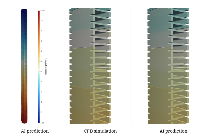
Figure 6 - Visualization of the kinematic pressure result for the Zig-Zag winding. We can see a good match between simulation results and AI predictions. You can recognize the washer positions in the zoomed-in view as slits
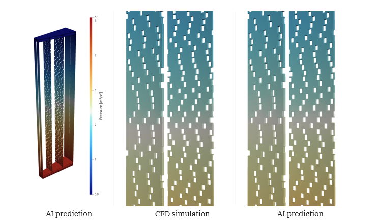
Figure 7 - Visualization of the kinematic pressure result for the axial channel winding. The holes that can be seen in the channels depict the position of the clack bands. We see a very good agreement between ground truth and predictions. Even the small pressure variations below the clacks have been correctly predicted with only minor deviations
Velocity Magnitude Field Reconstruction for Axial Channel Cooled Winding
For the axial channel cooled winding, we have visualized the velocity field to analyze whether the model has the ability to resolve the local flow features that are induced by the complex geometry of the spacers and clack bands. Figure 8 shows that the surrogate model indeed correctly identifies regions of high velocity. Note that it also provides good predictions in the narrow gaps between clacks. The flow patterns—visualized by the blue (low velocity) and orange/red (high velocity) regions—are morphologically identical to the reference CFD solution.
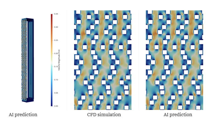
Figure 8 - Velocity in axial channel only windings. The left shows the cropped winding, where only the outer axial channel is visible. The right shows a zoomed in slice from the middle of an axial channel. Observe the good agreement between simulation and model prediction, in particular in the small channels created between adjacent clacks
This qualitative evidence suggests that the model generalizes well across different geometries, effectively learning the physics of fluid flow through the specific constraints of axial cooled channel winding designs.
5.2. Validation of Point-Wise Fidelity
To verify our first impression from the qualitative analysis, we computed error metrics to accurately assess the local accuracy of the model. For this, we computed the relative error at every spatial point within the domain. To do this robustly while mitigating the impact of numerical outliers at singular points, we report the 95th percentile of the relative error per sample. These metrics confirm that the model transcends simple scalar regression of the global pressure drop, accurately reconstructing the full pressure field throughout the winding geometry. For the Zig-Zag winding, on average, the 95% quantile relative point-wise difference between the surrogate model predictions and CFD numeric predictions is 1.9%. Likewise, for the axial channel cooled winding, the 95% quantile relative point-wise difference is 2.02%.
5.3. Validation of Global Pressure Drop Prediction
The global pressure drop, defined as the difference between the kinematic pressure at the top and bottom of the winding, is a critical parameter for pump dimensioning. For this reason, we now evaluate the model’s performance in predicting this global pressure drop. Figure 9 shows the strong correlation between the model predictions and the CFD results for both winding types. To quantify the error we use a relative metric per sample defined as: , where p is the global pressure drop. This results on the test set for the Zig-Zag winding in an error of 1.9% and for the axial channel cooled winding in 2.19%.
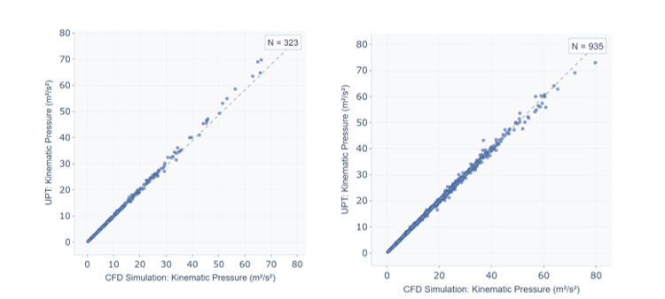
Figure 9 - Correlation plots of the kinematic pressure drop predictions and the CFD simulation results for the Zig-Zag winding (left) and the axial channel cooled winding (right) across the test set
5.4. Pressure Drop Characteristic Curves
For the design process of a transformer, the full pressure-flow characteristic per winding is necessary for the design of the flow distribution. Due to the very fast calculation time, it is possible to get the characteristic curves for a certain fluid from the machine learning model. Figure 10 shows examples of characteristic curves for the two winding types with commonly used cooling fluids. To ensure accuracy, we included verification points governed by full CFD simulations. These show excellent agreement with the UPT model prediction for the pressure-flow characteristics.
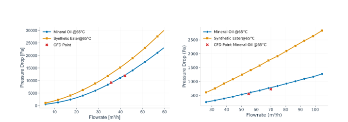
Figure 10 - Pressure-flow characteristic for Zig-Zag (left) and for the axial channel cooled winding (right) at 65°C for mineral oil and synthetic ester