Co-simulation Management Algorithm for Distribution System Operation with Real-Time Simulator
Authors
C. DIAZ-LONDONO - Dipartimento di Elettronica, Informazione e Bioingegneria, Milan, Italy
G. FAMBRI, A. MAZZA, E. PONS, M. BADAMI, E. BOMPARD, G. CHICCO - Dipartimento Energia “Galileo Ferraris”, Politecnico di Torino, Turin, Italy

Summary
This article presents a co-simulation framework consistent with the real-time simulation for operational analysis of electrical distribution networks. Realtime simulators have become a fundamental tool for testing and optimising control strategies in a safe and controlled environment. The proposed methodology outlines the steps required for setting up, controlling, and monitoring an electrical grid using a real-time simulator. The framework proposes the use of the Message Queuing Telemetry Transport communication between the electrical grid module and an external coordinator. An algorithm based on the Python programming language is proposed to manage the real-time simulation, create the grid topology, and communicate with the external coordinator. The implementation of the electrical network and the validation of the real-time simulator network are also presented. The article concludes that the proposed framework can improve the performance and flexibility of co-simulation for studies on the penetration of power electronics-based renewable sources.
Keywords
Electrical network - Renewable Energy Sources - Coordinator1. Introduction
Co-simulation with Real-Time (RT) simulators is becoming an essential tool for analysing and optimising electrical networks, including power system models. RT simulators accurately replicate the behaviour of power systems, allowing engineers to test and optimise control strategies in a safe and controlled environment. Various Hardware-In-the-Loop (HIL) testing systems have been developed based on RT simulators, such as the HIL-based high voltage ride-through and low voltage ride-through automated test system for photovoltaic inverters [1]. Other studies have explored the use of fieldprogrammable gate arrays [2] and LabVIEW RT and MATLAB/Simulink [3] for RT simulation and closed-loop testing of power system models.
Recent developments have led to the creation of Cyber-Physical Power System (CPPS) test-beds, specialised platforms for testing and validating the security and reliability of power grids. For example, a comprehensive review of future CPPS test-beds for securing electric power grids is provided in [4]. A RT-based platform for integrating power-to-gas in electrical distribution grids is proposed in [5], demonstrating the potential of co-simulation for optimising renewable energy integration. The challenges of latency and simulation stability in a remote power HIL co-simulation test-bed are addressed in [6], highlighting the importance of RT performance in these systems. The contribution [7] proposes an RT hybrid simulator of the distribution network, outlining the requirements for such a system. A versatile simulator for multiprocessor RT systems is developed in [8].
Moreover, researchers have developed new algorithms and frameworks to improve co-simulation performance and flexibility. A RT framework for heterogeneous software co-simulations is proposed in [9], which is able to provide an API that is based on a publish/subscribe mechanism. A flexible co-simulation framework for penetration studies of power electronics-based renewable sources is proposed in [10], featuring a new algorithm for phasor extraction. An efficient GPU-based electromagnetic transient simulation for power systems with thread-oriented transformation and automatic code generation is presented in [11]. In [12], a multi-platform RT microgrid simulation test-bed with hierarchical control of distributed energy resources featuring energy storage balancing is developed.
Recent studies have also demonstrated the potential of RT simulation for optimising the operation of integrated electricity and heat systems [13], and proposed remote HIL approaches for microgrid controller evaluation [14]. The paper [15] introduced a geographically distributed RT digital simulation approach using linear prediction, providing a promising solution for remote RT co-simulation. Furthermore, in [16] a RT simulation platform to support large-scale renewable energy access to the power grid is designed, whereas in [17] a co-simulation framework for transactive energy markets is proposed.
This article is based on the ideas presented in reference [5], properly updated and extended. A methodology is proposed for developing electrical grids using an RT simulator, outlining the steps required for its setup, control, and monitoring from an external coordinator. The necessary tools are described, including the information for their implementation. Furthermore, a framework is proposed for performing co-simulation analysis by using the Message Queuing Telemetry Transport (MQTT) communication between the electrical grid module (which takes into account the RT simulator) and the external coordinator. To control the electrical network simulator, an algorithm named PySimRT based on the Python programming language is proposed, which can create the grid topology, manage the RT simulation, and communicate with the external coordinator, among other functions. To validate the implemented network, the results are compared with those obtained by using a classical power flow solver for electrical distribution systems as the benchmark.
The paper aims to become a valid reference to enable all the players involved in the electrical distribution system analysis and simulation to handle the issues that may arise using the RT simulation approach, as well as provide a tested approach to enable the implementation of a co-simulation with proper management of the grid information. The proposed framework offers several key advantages, the primary one being the ability to simultaneously utilise multiple heterogeneous software tools. This eliminates the need for co-simulation partners to acquire additional licenses or share their proprietary models. By leveraging this approach, different software packages can seamlessly work together, enabling efficient collaboration without any unnecessary barriers. Another significant advantage is the relatively easy implementation of the PySimRT algorithm to manage the electrical network co-simulation. This algorithm simplifies the entire co-simulation process, including initialisation, simulation, and the obtaining of results. Its userfriendly nature makes it accessible and ensures smooth integration of the various components involved in the co-simulation.
The rest of the paper is organised as follows. Section 2 presents the proposed operational analysis framework, considering its main features, the developed algorithm, the operational modes, and the communication protocol used. Section 3 shows the implementation of the electrical network. In Section 4, the results obtained in the network implemented in the RT simulator are validated through the comparison with the results obtained with the backward/forward sweep solver. The last section contains the conclusions.
2. Description of the Operational Analysis Framework
This section aims to present the proposed operational analysis framework, considering its main features, the developed algorithm, the operational modes, and the communication protocol used.
2.1. General Description
The electrical network is implemented in an RT simulator, at the Global Real-Time Simulation Laboratory (G-RTS Lab), at Politecnico di Torino, Italy. The complete electrical network simulator module is presented in Figure 1. This module considers different software such as Python, MATLAB, Simulink, and RT-LAB, which are in constant communication when running the simulation. The module considers the hardware of the RT Simulator. In particular, an OPAL-RT Technologies simulator is considered with its RT-LAB platform. This platform implements the RT simulation of models directly from Simulink and takes into account MATLAB functions. The network module can be set and controlled from an external platform (named External Coordinator in Figure 1), i.e., a computer that runs in another geographic location. Indeed, this platform is appropriately designed to be executed in a co-simulation structure with different components. Therefore, in the module, it can be seen that the Python algorithm manages the communication between the external coordinator and the RT-LAB platform.
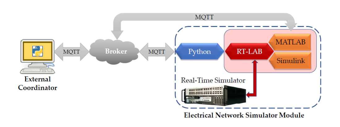
Figure 1 - Co-simulation structure
2.1.1. Main Features
The proposed framework offers several advantages considering a minimum user intervention. The main features are:
- The possibility to be executed and commanded locally or through an external coordinator.
- Bilateral wireless communications carried out with the external coordinator.
- Co-simulation structure that allows adding different assets to any node of the electrical network without modifying the network, sending the assets demand through the coordinator.
- Simulation performed in RT or considering different time steps.
- Different electrical networks can be generated creating several scenarios, i.e., the number of electrical nodes can be selected based on a predefined network.
- Different load consumption and Renewable Energy Sources (RES) profiles can be imposed, considering time slots of 15 min or 1 h.
- The user may upload their own consumption and RES profiles or work with the default profiles.
- The simulations can be run with different simulation horizons.
- Each node and transformer of the network has a monitoring system able to measure phase voltage, instantaneous current, instantaneous voltage, voltage in p.u. (per unit), active power (P), and reactive power (Q).
Moreover, the framework produces important outcomes for analysing the electrical networks, such as i) the grid losses, ii) the Reverse Power Flow (RPF), iii) the voltage profiles, iv) the line loading profiles, and v) the network power profiles. These outcomes enable the user to assess the network balances, the load of the lines, and the voltage operation. In addition, the line losses are useful to understand possible locations to install RES and achieve losses reduction. Likewise, the RPF provides relevant information for characterising and locating an asset to be installed in an electrical node. Regarding the assets that can be connected to any node of the grid, these include Power-to-Gas systems, enabling the linkage between electrical and gas networks [18], as well as Power-to-Heat systems, facilitating the integration of district heating networks with the electrical grid [19], among other possibilities.
2.2. Communication Protocol of the Module
The communication protocol implemented to carry out the communication between the electrical network module and the external coordinator is the MQTT protocol. In the MQTT protocol architecture, it is possible to identify three different network entities, as presented in Figure 2: the client publisher that sends messages, the client subscriber that receives the messages, and the broker that routes all the messages of the publishers to the different subscribers. In an MQTT communication architecture, multiple client publishers and client subscribers can coexist. If a client publishes and receives messages, it will be a publisher and a subscriber at the same time.
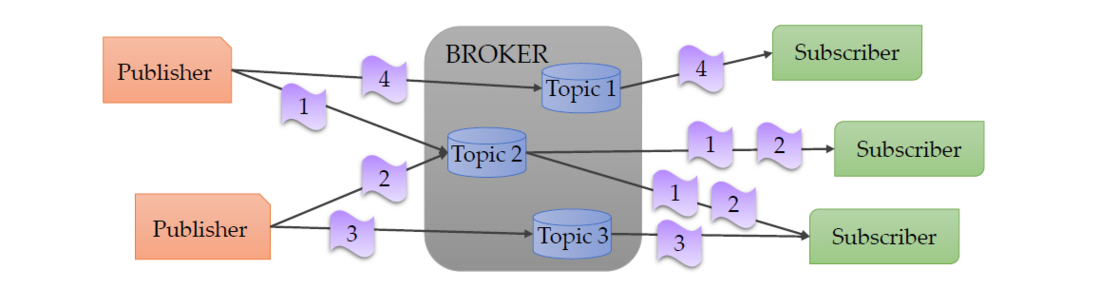
Figure 2 - MQTT publish/subscribe messaging protocol
In order to correctly dispatch the exchanged messages, the MQTT protocol organises the messages depending on their topics. When a publisher sends a message, it must define the topic to which the message belongs. The broker receives the message and saves it with the defined topic. Similarly, when a subscriber wants to receive a message, it must define the topic to which the message belongs and, when a message is published in that topic, the broker routes the message to the subscribed client. In this way, to carry out the communication, each client (whether a publisher or a subscriber) must only have knowledge of the used broker and of the topic of the messages concerned, without additional information regarding the client with which the message is being exchanged.
In order to build the MQTT communication architecture, the connection to the broker is done during the initialisation, by means of an MQTT library, declaring the topic/topics used for the communication. After this step, the messages are automatically exchanged until the clients stop publishing messages.
2.2.1. Communication with MATLAB/Simulink
The proposed MQTT communication method guarantees that all packages arrive to the clients (i.e., the electrical network and the external coordinator).
The data communication from the broker to the electrical network (Simulink models) is performed using the MQTT MATLAB toolbox. In fact, the initialisation of the Simulink models is done by a MATLAB routine that runs before starting the simulation. This routine contains the commands for connecting to the broker and subscribing to the topic/topics from which the model will receive data.
Moreover, a callback function is defined for every subscribed topic; therefore, whenever a new message arrives from the subscribed topic, the corresponding callback function is activated. The function receives as input the message exchanged through the MQTT protocol, extracts the required data, and passes them to the Simulink model.
The publication of the data generated by the models takes place through a MATLAB function inside a Simulink block. This block enables the use of external MATLAB functions and then to access the MQTT MATLAB toolbox. The function elaborates and prepares the data in the correct publication format (e.g., an ordered vector or a JSON format message) and publishes them in the prefixed topic.
2.3. Implementation of the PySimRT Algorithm and Operation Modes
In this subsection, the proposed algorithm developed in Python for the simulation on RT and the operation modes of the implemented framework are presented. This algorithm, named “PySimRT” enables the electrical network model to provide flexibility and scalability to achieve different complex RT simulation applications.
In order to launch the electrical network module, the PySimRT algorithm has been implemented and executed. A flow-chart of this algorithm is presented in Figure 3, in which a starting part and three modes are considered, i.e., initialisation, simulation, and results modes. The PySimRT implementation presented in Figure 3 considers different colours written as blue boxes for setting the RT simulator, green boxes for Python function statements, orange boxes for MQTT communications, grey boxes containing other boxes as routines carried out in RT platform or MATLAB / Simulink, yellow boxes for MATLAB functions, and red boxes for defining that the simulation is finished. In addition, the ellipsoids represent the steps that the external coordinator should command. For the sake of clarity, only the RT simulator commands (blue boxes) are presented explicitly.
Then, the starting part routines are:
- Import the required libraries such as the RT platform API (for interacting with the RT simulator) and MQTT client class (for performing the wireless communication), among others.
- Select the project that contains the predefined Simulink model.
- Define the Broker and the initial parameters and variables.
- Subscribe to the MQTT topics where the external coordinator can publish the information and run the different modes.
After the starting part, the PySimRT algorithm remains on stand-by, waiting for a message from the external coordinator, i.e., the algorithm is ready for executing the initialisation mode, commanded by the coordinator. Indeed, the following steps are separated into three different modes that are identified with different message topics and follows a specific sequence. Then, the electrical network modes are explained in the following subsections.
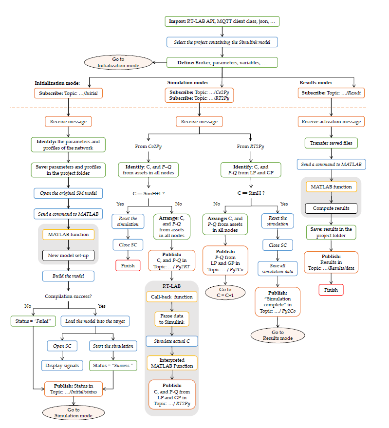
Figure 3 - Flow-chart of the PySimRT algorithm
2.3.1. Initialisation mode
This mode aims to set up the simulation parameters and leaves the simulation running and ready for the external coordinator to execute the cosimulation. Therefore, the coordinator builds a message that defines several aspects such as the simulation horizon (SimH), the grid topology (considering the node activation/deactivation), as well as the load and RES time-series. After the message arrives in the PySimRT algorithm, the RES profiles, load profiles, and grid line parameters (length, resistance, inductance, and maximum current) are saved in the project folder. Subsequently, the algorithm executes the following RT platform actions:
- Open the model.
- Execute a function entrusted with setting the grid nodes, i.e., the function activates and deactivates the chosen nodes.
- Compile the model, sending the electrical grid model to the RT simulator machine, and leaving the visualisation display in the RT platform interface.
- Start the electrical network RT simulation with the step counter (C) as zero, i.e., the simulation runs but does not update the data for the first step until the coordinator sends the counter value.
Finally, the PySimRT algorithm sends to the coordinator an initialisation status such as “Success” if all the process was developed or “failed” if the compilation process was not completed.
2.3.2. Simulation mode
This mode aims to perform the co-simulation from step one up to the simulation horizon SimH. The PySimRT algorithm can receive messages from the Coordinator (Co2Py) or from the RT simulator (RT2Py). Therefore, from the Co2Py, the PySimRT algorithm receives as input the Counter (one value), the active P and reactive Q power (two values per each node) demanded from additional assets attached in the network (if they are considered). Therefore, when the external coordinator sends a message through the MQTT protocol to the PySimRT algorithm, this message is encoded and sent as an array to MATLAB through the MQTT communication (in Py2RT). Subsequently, this array is sent to the RT platform. The simulation executes step C and sends an MQTT message (in RT2Py) to the PySimRT algorithm with P and Q of all the nodes. The algorithm receives from RT2Py the output message of the RT simulator, i.e., the unbalance matrix, and sends it to the external coordinator.
Moreover, when the counter C is equal to the simulation horizon SimH meaning the end of the co-simulation, the PySimRT algorithm stops the simulation. At this moment, the electrical network variables are saved in the folder project for later calculating the results.
In this mode, the external coordinator is responsible for exchanging power data from different assets or renewable energy sources connected to any node of the electrical network. Various requests for power absorption or injection may arrive at the coordinator from other platforms involved in the cosimulation. The coordinator then makes decisions on managing the power of each asset, considering its constraints and the electrical network constraints. Notice that the co-simulation partner executes the requested power for the asset based on its preferences, while the RT simulator responds with the electrical network’s behavior.
2.3.3. Results mode
This mode aims to compute the electrical network outcomes. The PySimRT algorithm receives an activation message that enables the calculation of the results. This activation message is sent at the end of the simulation mode after the data has been saved. After the enable message arrives, the script reallocates the network variables saved in a “Results” folder. Then, a function entrusted with computing the results based on the saved data is executed. Subsequently, these results are returned to the script and sent by an MQTT message to the coordinator (see Figure 1). The computed results are grid losses in % and kWh, reverse power flow in MW, voltage profiles in p.u., line loading in A, and grid power in MW.
3. Electrical Distribution Network
In this section, the electrical network implemented in the proposed framework is presented. The presentation starts by indicating the network features for later introducing the simulation implementation in the RT simulator.
3.1. Network Description
The electrical network considered is based on a portion of a Medium-Voltage (MV) grid topology of Turin (a city in North-Western Italy). This network has five feeders derived from three 22 kV busbars of a 220/22 kV primary substation at a frequency of 50 Hz, feeding 43 Medium-Voltage/Low-Voltage (MV/LV) substations as presented in Figure 4.
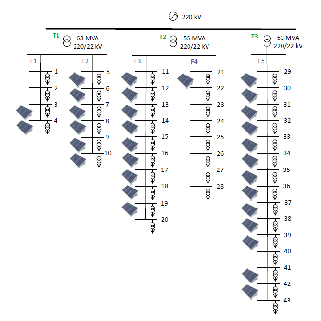
Figure 4 - Topology of the electrical network with PV generation
3.2. Simulation Deployment
The electrical network is implemented in the RT-LAB platform which is the built-on software of OPAL-RT Technologies. The network is developed considering the methodology presented in [5], in which the RT platform implements the RT simulation of models directly from Simulink. Then, the model is deployed in Simulink following a two-subsystems scheme, i.e., the Subsystem of the Console (SC) and the Subsystem of the Master (SM). In addition, a model initialisation block for charging the grid parameters and required libraries are considered.
3.2.1. Subsystem of the Console
The SC considers the user interface of the model as well as the MQTT communication deployment. In the SC, the main output variables are depicted, such as the total network power consumption or the voltages at each node of the feeders. Then, this subsystem contains:
- Visualisation: displays the signals generated during the simulation. These display blocks depict time-domain signals with respect to the RT fixed in the simulation.
- Monitoring: this information refers to the computation time, the RT size, and the number of overruns.
- MQTT communication: it is carried out by two blocks, one for receiving and other for sending data.
- Subscribe: This block acquires the counter value (simulation step), which is commanded by the coordinator. This block allows receiving additional power demand (e.g., from an asset).
- Publish: This block sends the load and renewable generation data of each node at each simulation step.
3.2.2. Subsystem of the Master
The SM considers the different interconnections with the electrical network, in which all computational elements, mathematical operations, and signal generators are implemented. The integration of these components is presented as follows:
- Electrical network: the distribution electrical network receives the load and generation profiles, i.e., the aggregated electrical demand and renewable generation profiles in each node. These load profiles consider the passive load and possible asset demands. Notice that adding assets to the grid affects only the power flow and not the grid topology, because the asset are basically represented as components exchanging power (i.e., PQ components). As a result, the grid structure is always represented with the same impedances, while the assets modify the load in the connected nodes.
- Uncontrollable nodal loads and renewable generation profiles: data of different users and RES generation is provided every time step (e.g., 15 or 60 minutes) to each node of the network.
- Monitoring block: contains an RT platform block that provides information on model timing‘, i.e., computation time, RT size, and numbers of overruns.
- Save data: the data is saved in RT commanded by a triggered pulse for acquiring specific periods of time.
3.2.3. Electrical Network Integration
The electrical network is considered inside the SM, and is modeled with three-phase elements. This model considers i) the transmission system, in which the High Voltage (HV) level is represented by a Th´evenin equivalent; ii) measurements systems able to report the phase voltage, the instantaneous current and voltage, the voltage p.u., and the active and reactive powers; iii) HV/MV transformers (T1, T2, and T3); and, iv) five feeders considering every single node. In addition, the inputs of the node are the three-phase voltages and currents as well as the load and renewable generation profiles. Measurement systems are implemented in all the nodes of the network for monitoring purposes. The distribution lines are implemented as a lumped -model of a balanced three-phase distribution system. Finally, it is assumed that the voltage at the slack node remains constant. In such a scenario, there would be no requirement for a tap changer.
3.3. Electrical Network Stabilization Time
To determine the grid stabilization time, and understand the minimum time required to input new data from uncontrollable power profiles into the model, a voltage stabilization analysis was conducted. The analysis considers a sample time of 15 minutes (i.e., steady state). The highest data jump (i.e., the difference between the magnitude of two consecutive data points) within the load or renewable generation profiles is considered.
Then the model is run by focusing on the time period surrounding the highest data jump detected. During this simulation, new values from lookup tables (power profiles) are fed into the simulation every second, in which every second represents the scenario time interval of 15 minutes. Consequently, the electrical network experiences disturbances from new data every second, leading to voltage quality distortion. Then, the question is: how much of this second is required to stabilise the simulation?
Figure 5a presents the three-phase voltage at the node with the largest deviation. In the second 2, the highest data jump occurs, and the distortion of the signal is slightly noticeable. Figure 5b and Figure 5c show zoomed-in views of Figure 5a (purple and green rectangles) to provide clarity on these disturbances.
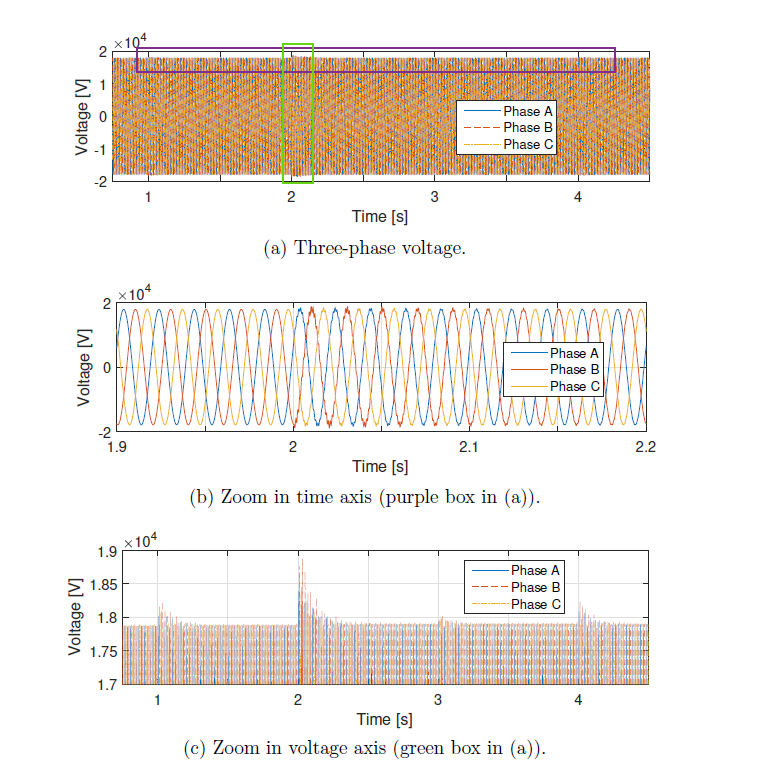
Figure 5 - Three-phase voltage at a node after feeding data
To establish an acceptable disturbance level in the voltage signal, the Total Harmonic Distortion (THD) is used as the metric parameter. Figure 6 depicts the THD of the voltage signal mentioned earlier. For this research, a THD≤0.2% is considered acceptable, indicating that the voltage at fundamental frequency (i.e., 50 Hz) is well represented by the signal. Phase B exhibits the highest THD and, consequently, the longest stabilization time, reached in less than 400 ms.
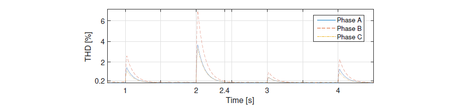
Figure 6 - Total Harmonic Distortion of the node voltage
4. Electrical Network Validation and Case Study
The electrical network implemented in the RT simulator is validated through the comparison of the results obtained in the proposed PySimRT framework and the results provided by the Backward/Forward Sweep (BFS) algorithm [20]. The BFS solves the power flow equations and is particularly suitable to solve radial distribution systems. The validation is carried out with two different case studies. Therefore, the electrical network is set up and commanded by an external coordinator platform (not in the G-RTS Lab) considering the operation modes presented in Section 2.3. These case studies are performed with the default values.
4.1. Current and Grid Losses Computation from the PySimRT
The network model is represented through the branch-to-node incidence matrix , in which the rows refer to the branches b = {1, ...,B} and the columns to the nodes n = {1, ...,N − 1} (slack node excluded). For each branch, the column corresponding to the initial node of the line contains the value 1, while the column corresponding to the ending node of the line contains the value -1. All other entries are equal to zero. Moreover, the matrix
is defined as the inverse of the branch-to-node incidence matrix L, i.e.,
(1)
For a specific branch b = {1, ...,B}, the electrical grid parameters such as resistance Rb and reactance Xb are required for obtaining the branch impedance Zb as
Zb = Rb + j Xb, (2)
where, the resistance Rb, and the reactance Xb are computed as and
, respectively. Here,
is the unitary resistance (in Ω/km) and
is the unitary inductance (in H/km) of the branch, and lb is the branch length (in km).
With the purpose of computing the losses and the line loading, the currents flowing in the branches are calculated. Therefore, for computing the currents in the branches referring to the simulation developed in the PySimRT algorithm, the following analysis is established.
Three phase-to-ground voltages are taken and recorded from the Simulink simulation file. In fact, the data are acquired when the electrical grid is in a steady state (before the demand power changes) at every time step (representing for example 15 minutes). However, it should be noted that the RT simulator operates in electromagnetic transient (EMT) mode with a selected sample time of 250 μs. As a result, at each time step, steady-state data is recorded, resulting in approximately 2000 records between 500 ms and 1 s after reaching a steady state. Therefore, any demand power changes could be made rapidly, ideally every second, to ensure accurate simulation results and responsiveness to dynamic system conditions. Then, the three voltages are measured in each node and in the slack node, which is considered to be the MV side of the HV/MV transformer. In order to compute the current in each branch, the time difference Δt between the slack node voltage and the voltage at each node is needed for later calculating the voltage angle. Then, the time difference Δt is estimated by the successive process. Figure 7a presents an example of the ideal three-phase voltage measurement in the slack node (continuous lines) and in another node (dashed lines). In this research, the times are compared when the signals are going upward and cross zero (see red box in Figure 7a). Moreover, in Figure 7b, a zoom of Figure 7a is presented (zoom around the red box), where the time difference of the voltages when crossing zero can be seen.
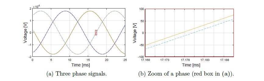
Figure 7 - Three phase voltage in the slack and in another node
However, the actual voltage measurement is given with a sample time of 250 μs, providing a stair-wise performance as presented in Figure 8a. Likewise, Figure 8b depicts a zoom of Figure 8a (zoom around the red box), and differently from Figure 7b where the time difference between the voltages is clearly noticed, in this discrete voltage response the time difference is not well defined. To address this aspect, the sine discrete voltage is interpolated. Therefore, 200 points between each measured point are generated for increasing the voltage times resolution, obtaining the performance presented in Figure 9a. Subsequently, the two points closest to zero are identified per voltage profile with the purpose of calculating linear functions. These functions are evaluated with the voltage equal to zero to obtain the crossing zero time (see the green points in Figure 9b). Then, the difference is computed for the three phases of all nodes.
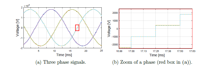
Figure 8 - Measured three phase voltages in the slack node and in another node
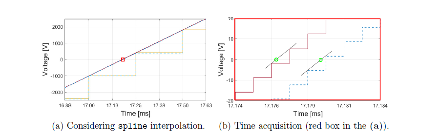
Figure 9 - Voltage phase measured in the slack and in another node
After computing Δt and considering f = 50 Hz, the angle ϕn in radians is calculated as
(3)
Thus, the complex nodal voltage , whose amplitude is a Root Mean Square (RMS) value generated as
(4)
For the network calculations, starting from the base power Sbase (i.e., the three-phase apparent power) and from the base voltage Vbase (i.e., the RMS phase-to-phase voltage), the base current Ibase and the base impedance Zbase are determined as
(5)
The calculations are then carried out in per units, returning to the RMS values after the results have been obtained. In vector terms, the complex node currents and the complex branch currents, expressed in per units, are included in the vectors and
, respectively. The complex node current vector is defined as the sum of the load currents
(for all the loads connected to a given node) and of the currents
flowing in the shunt components of the π-model of the lines that converge to the same node:
. (6)
In particular, considering the node load complex power vector for all the nodes, and considering the node complex voltage vector
, the corresponding node complex current vector
and the currents in the shunt
are written as
(7)
where is a vector computed as the sum of the load admittance vector
and the network shunt admittance vector
at each node:
(8)
The vector is computed by taking into account, at each node, one half of the shunt admittance in the π-model of each line that converges to the node:
(9)
where, by considering the unitary capacitance cb (in F/km) that forms the shunt admittance vector and the line length lb (in km) of the lines b = 1, ..., B:
(10)
Thus, the complex branch current vector ib is defined as:
, (11)
where, the mathematical operators ◦ and ⊘ are the Hadamard product and division, respectively [21].
The current in[A] and ib[A] vectors, with values expressed in [A], are then respectively computed as:
(12)
(13)
Finally, the grid losses in per units and in [W] are respectively expressed as:
(14)
(15)
4.2. Validation Cases
The validation of the electrical network power flow is developed by comparing electrical indices computed with the proposed PySimRT algorithm and the classical BFS algorithm. These indices are calculated starting from the grid losses, the line loading, and the voltage profiles. The losses and line loading are computed after the simulation completes the data acquisition in the entire horizon. Then, two cases are assessed: a base case without PV production and the second one with PV production as indicated in Figure 4, where 31 over 43 nodes host PV production.
The PySimRT default case is simulated, in which the total passive load installed power is 35.66 MW, divided among different types of users, i.e., residential, industrial, commercial, and offices. The data used in this study are obtained by considering the real load nominal power and real power profiles of this Turin electrical network portion. The details regarding the installed power of every type of load per feeder are shown in Table 1.
| Feeder | Residential [MW] | Industrial [MW] | Commercial [MW] | Office [MW] | Total [MW] | PV [MW] |
|---|---|---|---|---|---|---|
| 1 | 0.33 | 0.25 | 0.33 | 0.12 | 1.02 | 1.24 |
| 2 | 1.25 | 1.25 | 2.35 | 0.65 | 5.46 | 6.65 |
| 3 | 4.16 | 1.94 | 3.52 | 1.98 | 11.60 | 10.02 |
| 4 | 2.40 | 1.62 | 4.16 | 0.86 | 9.05 | 2.00 |
| 5 | 4.49 | 1.09 | 1.35 | 1.61 | 8.53 | 8.43 |
| Whole grid | 12.63 | 6.11 | 11.71 | 5.21 | 35.66 | 28.34 |
4.2.1. Base Case
Regarding the grid daily energy losses, PySimRT reports 288.48 kWh, whereas the BFS algorithm reports 288.51 kWh. Figure 10 depicts the losses in each transformer (i.e., T1, T2, and T3), comparing both solutions. The line before connecting node 21 (T2) is the one with the largest losses, achieving 5.36 kW at 8:30 for both solutions, while the line connecting node 4 is the one that reports the smallest losses, reaching 1.04 W at 2:45 for both solutions (not presented in Figure 10).
The loading factor response in PySimRT and BFS is depicted in Figure 11. In fact, the figure depicts the maximum line loading profiles per each transformer. The peak current is 66.8 A corresponding to 19.6% loading) at 8:30 in the T2 for both solutions, the difference between them is 8.9×10⁻³ A.
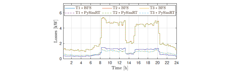
Figure 10 - Maximum grid losses per transformer (Base case)
The lines before connecting nodes 11, 12, 21, and 22 have the highest loading levels, reaching values higher than 17%. These lines correspond to the nearest one to T2 in feeders 3 and 4 (F3 and F4 in Figure 4). On the other hand, the less loaded lines (not presented in the figure) supply nodes 4, 10, and 43, i.e., the last line in the transformers 1 and 3 in feeders 1, 2, and 5 (F1, F2, and F5 in Figure 4).
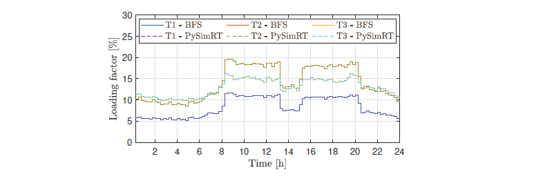
Figure 11 - Line loading for both algorithms in each transformer (Base case)
Regarding the voltage profiles of the PySimRT and BFS algorithms, Figure 12 presents the p.u. profiles. In Figure 12a the maximum voltage per transformer is depicted, in which the maximum value is 1.0011 p.u. for PySimRT and 1.0014 p.u. for BFS, in both cases it is at 4:30 in node 30 (T3); then the difference is 3.0 × 10⁻⁴ p.u. The nodes from 29 to 35 (first nodes in F5, i.e., T3) have the highest voltage levels. Whereas, Figure 12b shows that the minimum value is 0.9953 p.u. for PySimRT and 0.9952 p.u for BFS, in both cases it is at 8:45 in node 28 (T2); the difference is 2.0×10⁻⁴ p.u.
In fact, the minimum voltages are reported at T2. Notice that the voltage profiles are relatively flat and there is no overvoltage.
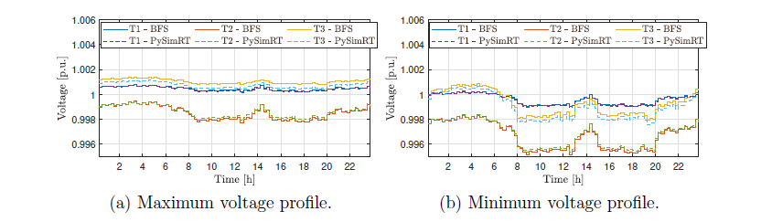
Figure 12 - Voltage per unit for both algorithms in each transformer (Base case)
4.2.2. Case with PV production
The grid daily energy losses in the second simulation are presented in Figure 13. In fact, PySimRT reports losses of about 226.01 kWh, whereas the BFS algorithm reports 226.04 kWh. Notice that in this case, the grid losses are lower than in the base case, while the differences between the algorithms are similar. Moreover, as in the previous case, the line supplying node 21 (T2) is the one with the largest losses, achieving 4.96 kW at 19:45 for both solutions.
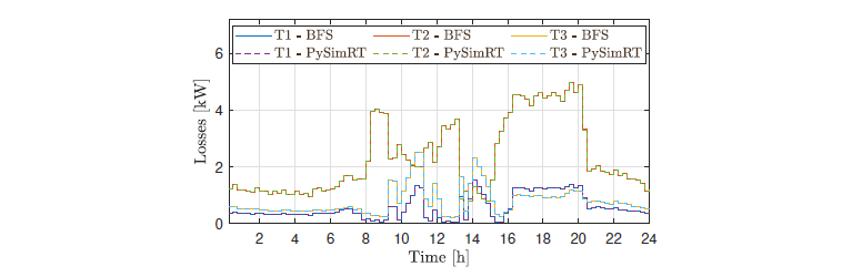
Figure 13 - Maximum grid losses per transformer (Case with PV)
Figure 14 presents the line loading response. It depicts the maximum line loading per transformer. The peak current is 76.7 A (corresponding to 22.5% loading) at 10:45 in T3 for both solutions, PySimRT and BFS, the difference 23 between them is 5.6 × 10⁻³ A. Notice that the transformer with the highest loading factor has changed due to high PV penetration in T3. On the other hand, the less loaded lines are the ones in T1, as in the base case.
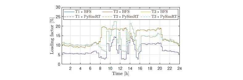
Figure 14 - Line loading for both algorithms in each transformer (Case with PV)
The voltages profiles of the PySimRT and the BFS algorithms are presented in Figure 15. In Figure 15a the maximum voltages per transformer are depicted, in which the maximum value is 1.0050 p.u. for PySimRT and 1.0052 p.u. BFS at 13:45 in node 38 (T3); then, the difference is 1.9 × 10⁻⁴ p.u. In fact, nodes in T3 have the highest voltage levels when considering PV production. Figure 15b presents the minimum value at 0.9955 p.u. for PySimRT and 0.9953 p.u for BFS, in both cases, it is observed at 18:15 in node 28 (T2); the difference is 2.0 × 10⁻⁴ p.u. In fact, the minimum voltages are reported in F4 (T2), where the PV production is considered in only one node. Notice that, again, there is no overvoltage.
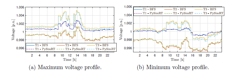
Figure 15 - Voltage per unit for both solutions in each transformer (Case with PV)
Finally, Table 2 summarises the validation indices for both algorithms.
| Case | Index | PySimRT | BFS | Difference |
|---|---|---|---|---|
| Base | Daily grid losses Peak current Max voltage Min voltage | 288.48 kWh | 288.51 kWh 66.8 A (19.6%) 1.0014 p.u. 0.9952 p.u. | 30 Wh 8.9 × 10⁻³ A 3.0 × 10⁻⁴ p.u. 2.0 × 10⁻⁴ p.u. |
| With PV | Daily grid losses Peak current Max voltage Min voltage | 226.01 kWh 76.7 A (22.5%) 1.0050 p.u. 0.9955 p.u. | 226.04 kWh 76.7 A (22.5%) 1.0052 p.u. 0.9953 p.u. | 30 Wh 5.6 × 10⁻³ A 1.9 × 10⁻⁴ p.u. 2.0 × 10⁻⁴ p.u. |
In fact, the differences in the evaluated indexes between the algorithms are negligible, achieving differences in the order 1 × 10⁻³ in the loading factor, and 1×10⁻⁴ p.u in the voltages. Moreover, It can be seen that after installing PV generation, the grid losses are reduced by 21.7%, the peak loading factor increases from 19.6% to 22.5%, and the maximum voltage rises around 4 × 10⁻³ p.u. In addition, the small errors in the analysed indices of PySimRT validate the adequate performance of the implemented model.
5. Conclusions
The interaction among different units of a co-simulation system requires the knowledge of the technical characteristics of each unit, the structure of their interface, and the potential of using each unit with the available data. In this paper, the units involved have been the traditional power flow implementation with the BFS solver and the Simulink implementation of the power flow calculations aimed at sending the data to an RT simulator.
The proposed methodology outlines the steps required to set up, control, and monitor an electrical grid using a real-time simulator. It proposes the use of MQTT communication between the electrical grid module and an external coordinator. An algorithm, named PySimRT, based on the Python programming language, is proposed to manage the real-time simulation, create the grid topology, and communicate with the external coordinator.
The framework’s primary advantages include the ability to use multiple heterogeneous software tools simultaneously, eliminating the need for additional licenses or model sharing. It offers a user-friendly approach for co-simulation, simplifying the entire process, from initialization to obtaining results. The proposed methodology is validated by implementing an electrical network and comparing the results with a classical BFS power flow solver.
The BFS solver is a steady-state computation tool that does not depend on time. Conversely, the Simulink implementation applies embedded dynamics to reach time-varying solutions. Consistency has to be guaranteed between the two solvers, depending on the time step considered for the BFS and on the type of data used. If the data used for the BFS, e.g., with a time step of one minute, are intended as a stairwise evolution in Simulink, the Simulink calculations need to solve each minute a problem of step response for each variable and time step, whose dynamics depend on the internal settings of the functions in Simulink. Reaching the steady state from Simulink consistent with the BFS results depends on the data (in particular on the variations from one time step to the next one) and on the minimum time duration sufficient to run Simulink and have the final values close to the BFS results with a difference lower than the tolerance of the BFS iterative process. This minimum time duration is also the minimum time for which the data can be exchanged with an RT simulator to have consistent co-simulation and RT simulation outcomes.
This paper aims to serve as a comprehensive reference for the analysis and simulation of electrical distribution systems using real-time simulation. It provides a tested approach to co-simulation and offers efficient collaboration between different software packages without any unnecessary barriers. Future work will focus on proposing a matrix-based approach to enhance the methodology, streamlining the process of creating new networks. This will further improve the flexibility and usability of the co-simulation framework.
References
- F. Li, M. Liu, Y. Wang, X. Zhang, Research on HIL-based HVRT and LVRT automated test system for photovoltaic inverters, Energy Reports 7 (2021) 405 – 412. doi:10.1016/j.egyr.2021.08.026.
- W. Li, L.-A. Gr´egoire, S. Souvanlasy, J. B´elanger, An FPGA-based realtime simulator for HIL testing of modular multilevel converter controller, in: 2014 IEEE Energy Conversion Congress and Exposition (ECCE), 2014, pp. 2088 – 2094. doi:10.1109/ECCE.2014.6953678.
- A. Parizad, H. R. Baghaee, M. E. Iranian, G. B. Gharehpetian, J. Guerrero, Real-time simulator and offline/online closed-loop test bed for power system modeling and development, International Journal of Electrical Power & Energy Systems 122 (2020) 106203. doi:https://doi.org/10.1016/j.ijepes.2020.106203.
- R. V. Yohanandhan, R. M. Elavarasan, R. Pugazhendhi, M. Premkumar, L. Mihet-Popa, J. Zhao, V. Terzija, A specialized review on outlook of future Cyber-Physical Power System (CPPS) testbeds for securing electric power grid, International Journal of Electrical Power and Energy Systems 136 (3 2022). doi:10.1016/j.ijepes.2021.107720.
- C. Diaz-Londono, G. Fambri, A. Mazza, M. Badami, E. Bompard, A real-time based platform for integrating power-to-gas in electrical distribution grids, in: 2020 55th International Universities Power Engineering Conference (UPEC), 2020, pp. 1–6. doi:10.1109/UPEC49904.2020.9209803.
- E. Bompard, S. Bruno, A. Cordoba-Pacheco, C. Diaz-Londono, G. Giannoccaro, M. L. Scala, A. Mazza, E. Pons, Latency and simulation stability in a remote power hardware-in-the-loop cosimulation testbed, IEEE Transactions on Industry Applications 57 (2021) 3463–3473. doi:10.1109/TIA.2021.3082506.
- D. X. Morales, R. D. Medina, Y. Besanger, Proposal and requirements for a real-time hybrid simulator of the distribution network, in: 2015 CHILEAN Conference on Electrical, Electronics Engineering, Information and Communication Technologies (CHILECON), 2015, pp. 591– 596. doi:10.1109/Chilecon.2015.7400438.
- H. Anca, S. Gheorghe, RTMultiSim: A Versatile Simulator for Multiprocessor Real-Time Systems, in: 3rd International Workshop on Analysis Tools and Methodologies forEmbedded and Real-time Systems, 2012, pp. 1–6.
- J.-F. C´ecile, L. Schoen, V. Lapointe, A. Abreu, J. B´elanger, A distributed real-time framework for dynamic management of heterogeneous co-simulations, Opal-RT Technologies Inc., Montr´eal, Canada (2006).
- T. S. Theodoro, M. A. Tomim, P. G. Barbosa, A. C. Lima, M. T. C. de Barros, A flexible co-simulation framework for penetration studies of power electronics based renewable sources: A new algorithm for phasor extraction, International Journal of Electrical Power and Energy Systems 113 (2019) 419–435. doi:10.1016/j.ijepes.2019.05.047.
- Y. Song, Y. Chen, S. Huang, Y. Xu, Z. Yu, W. Xue, Efficient gpu-based electromagnetic transient simulation for power systems with threadoriented transformation and automatic code generation, IEEE Access 6 (2018) 25724–25736. doi:10.1109/ACCESS.2018.2833506.
- R. S. Mongrain, Z. Yu, R. Ayyanar, A real-time simulation testbed for hierarchical control of a renewable energy-based microgrid, in: 2019 IEEE Texas Power and Energy Conference, TPEC 2019, 2019, pp. 1–6. doi:10.1109/TPEC.2019.8662133.
- T. B. H. Rasmussen, Q. Wu, M. Zhang, Combined static and dynamic dispatch of integrated electricity and heat system: A real-time closedloop demonstration, International Journal of Electrical Power and Energy Systems 143 (12 2022). doi:10.1016/j.ijepes.2022.107964.
- K. Prabakar, A. Valibeygi, S. A. R. Konakalla, B. Miller, R. A. De Callafon, A. Pratt, M. Symko-Davies, T. Bialek, Remote hardwarein- the-loop approach for microgrid controller evaluation, in: 2020 Clemson University Power Systems Conference (PSC), 2020, pp. 1–8. doi:10.1109/PSC50246.2020.9131282.
- R. Liu, M. Mohanpurkar, M. Panwar, R. Hovsapian, A. Srivastava, S. Suryanarayanan, Geographically distributed real-time digital simulations using linear prediction, International Journal of Electrical Power and Energy Systems 84 (2017) 308–317. doi:10.1016/j.ijepes.2016.06.005.
- J. Shi, R. Zhang, L. Qu, H. N. Pan, K. Cui, L. Yin, X. Ma, X. Zhou, J. Cui, P. Wang, Design of a real-time simulation platform to support large-scaled renewable energy access to power grid, in: 18th International Conference on AC and DC Power Transmission (ACDC 2022), Vol. 2022, 2022, pp. 836–839. doi:10.1049/icp.2022.1298.
- D. Cutler, T. Kwasnik, S. Balamurugan, T. Elgindy, S. Swaminathan, J. Maguire, D. Christensen, Co-simulation of transactive energy markets: A framework for market testing and evaluation, International Journal of Electrical Power and Energy Systems 128 (6 2021). doi:10.1016/j.ijepes.2020.106664.
- G. Fambri, C. Diaz-Londono, A. Mazza, M. Badami, T. Sihvonen, R. Weiss, Techno-economic analysis of power-to-gas plants in a gas and electricity distribution network system with high renewable energy penetration, Applied Energy 312 (2022) 118743. doi:https://doi.org/10.1016/j.apenergy.2022.118743.
- G. Fambri, A. Mazza, E. Guelpa, V. Verda, M. Badami, Power-to-heat plants in district heating and electricity distribution systems: A technoeconomic analysis, Energy Conversion and Management 276 (2023) 116543. doi:https://doi.org/10.1016/j.enconman.2022.116543.
- D. Shirmohammadi, H. Hong, A. Semlyen, G. Luo, A compensationbased power flow method for weakly meshed distribution and transmission networks, IEEE Transactions on Power Systems 3 (2) (1988) 753–762. doi:10.1109/59.192932.
- R. A. Horn, C. R. Johnson, Matrix Analysis, Cambridge University Press, 1985. doi:10.1017/CBO9780511810817.