A multi-scale finite element beam-to-solid submodelling strategy to compute contact stresses in multi-layered stranded cables
Authors
S. JABORNEGG - EnDes Engineering, Switzerland
R. BAUMANN - Competence Center Mechanical Systems, Lucerne University of Applied Sciences and Arts, Switzerland
S. LANGLOIS, P.H.C. ROCHA - Department of Civil and Building Engineering, Université de Sherbrooke, Canada

Summary
The present work deals with the numerical computation of local stresses in multi-layered stranded cables typically used for overhead transmission line conductors. A multi-scale finite element strategy to compute the stresses in the vicinity of the contact zones between crossing wires of the two outermost layers is developed. This strategy is based on finite element (FE) beam models. Two submodelling steps shift the focus from a global to a local perspective. In the first submodelling step, displacements and forces are transferred from the beam model to a solid submodel. This submodel includes the entire cable cross section. Transferred displacements on one side stabilize the model but introduce an error due to the differences of beam and solid elements. However, result validity is ensured due to transferring of forces to the other side of the submodel. The second step is a local solid-to-solid submodel of one contact zone. Thereby, displacements are transferred from the first to the second submodel. The developed strategy is tested on single-, two- and four-layered stranded cable models. For validation, 3D FE solid models, including submodels, are used. The good correlation of the results, mainly contact forces and contact stresses, emphasizes the potential of the present strategy in computing local stresses in multi-layered stranded conductors with acceptable computation times.
Keywords
Cable Modelling, Contact Modelling, Finite Element Simulation, Overhead Conductors, Submodelling1. Introduction
Overhead conductors are important structural elements of transmission lines. In addition to carrying electrical energy, conductors are subjected to several mechanical loads that they should withstand while keeping their mechanical integrity over their lifetime. These mechanical loads have a quasi-constant component due to the mechanical tension and the clamping force, and a variable component due to oscillations in large parts caused by vortex induced vibrations. Due to its geometrical form - helical-shaped strands constructed in layers with different winding directions (see Fig. 1) - overhead conductors have thousands of contacting points between strands and between outer strands and accessories of the line (e.g. suspension clamp, spacers, dampers). At such contact regions (see Fig. 2) severe stress concentration arises and fatigue damage accumulates leading to possible fatigue failure of the strands especially in the vicinity of suspension clamps.

Figure 1 - Structure of a multi-layered helical strand
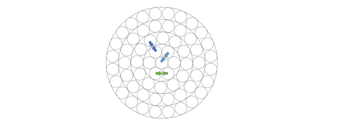
Figure 2 - Contact types occurring in a multi-layered helical strand
Fatigue damage in conductors is a local phenomenon proper to the points of contact over the strands [1], [2]. Therefore, an approach that considers the local stress effects of these points, where usually cracks initiate, is probably the best approach to handle this problem if one aims to investigate the local driving forces of the failure. Unfortunately, complexities related to the geometry of the conductor-clamp assembly, material behaviour and multiaxial stress distribution on the contacting points make the use of analytical approaches to tackle the fatigue problem from a local perspective extremely complex. In that sense, the use of analytical models is typically restricted to nominal fatigue indicators [3], [4]. As a result, investigations related to the fatigue behaviour of conductors have traditionally been based on experimental tests of conductor-clamp assemblies [5]-[8]. Tests of this type attempt to reproduce the static and dynamic loading that the conductor might be subjected to, but in a laboratory environment. Besides being expensive and technologically difficult to carry out, this type of test provides results based on nominal fatigue indicators only (e.g. tension load and vibration level) and does not reveal much about the local driving forces of crack initiation that lead the strands to fail.
Taking advantage of recent developments in numerical simulation tools and computer’s performance, several finite element (FE) models have been proposed to better understand the overall mechanical behaviour of conductors and to provide more information about the local driving forces generating fatigue damage. These FE-models can be divided into two main categories: models based on beam elements and models based on solid elements. Beam element models as proposed by Lalonde et al. [9], Baumann and Novak [10] and others [11]-[14] take advantage of the slender shape of conductors to model their strands using beam elements. Works using this approach exploit the reduced number of degrees of freedom of beam elements to develop longer length cable models and simulate more complicated loading histories, since the computational cost remains reasonable. Despite providing accurate results about the mechanical behaviour of the conductor and stress distribution along its strands, the major drawback of beam element models is the poor provision of stress concentration effects observed in the contact points along the strands which limits the computation of these stress effects on the fatigue damage evaluation. On the other hand, solid element models of conductors as proposed by [15]-[22] discretize the conductor strands into small portions using three-dimensional solid elements which enables the evaluation of the effects of the stress distribution in the vicinity of the contacting regions. These models can account for various local stress effects such as stress concentration, stress gradient and elastic-plastic deformations typical for contacting problems and fatigue damage. However, they easily reach a large number of degrees of freedom, which implies a large computational cost to solve these problems. Therefore, this approach is usually limited to short length cable models and low complexity loading histories. Moreover, the level of discretization generally achieved is, due to computational limitations, still coarser than the one necessary to compute the stress field distribution along the contacting regions with proper accuracy. Several previous studies show that elements of the size of a few micrometres are necessary to compute the stress distribution in the contact region of wires [1], [2], [23], [24]. In this context, an alternative that provides an accurate solution to the problem of contacts between cable strands and their stress field while keeping the computational cost reasonable becomes desirable when investigating the fatigue problem from a local perspective.
In terms of computational efficiency and accuracy, submodelling has proven to be a promising technique to handle the stress concentration and contact problems in FE analyses [24] - [31]. This technique consists of using the solution of a coarse mesh model as boundary conditions to a local and refined mesh model, that is generally limited to the region of interest. The work of Cormier et al. [31] is one of the first papers to use submodelling to solve contact problems. This paper establishes a new and effective criterion for evaluating the convergence of the submodel results by comparing the stress results at different mesh refinement levels. The work of Rajasekaran and Nowell [29] indicates that submodelling is an efficient approach to deal with contact problems. However, care should be taken when using the displacement based approach since errors have been observed when comparing the numerical results with an analytical model of the same contact problem. Other works point out that this problem is related to the difference of contact stiffness between the global and local models [26], [31], [32]. This problem becomes particularly evident when the displacement field of both models diverge, but it can be circumvented by using other contact algorithm approaches, e.g. Lagrange multipliers and Augmented Lagrangian. Curreli et al. [26] also propose that force based and stress based approaches can be used to solve the contact stiffness problem. The work of Elke and Sracic [30] points out that the size of the region of interest also plays an important role on the accuracy of the results of stress distribution. They conclude that the smaller the region of interest, the greater the errors in computing the contact stresses.
The study presented here aims to develop a multi-scale finite element strategy by using a submodelling approach to compute the local stresses in the contacts between the crossing wires of the two outermost layers of a stranded cable. The cables modelled reproduce the geometry of overhead transmission line conductors, but at this stage of the research, only steel material properties are modelled to avoid difficulties in the convergence and modelling of multi-material contacts. Starting with a global beam model, two levels of submodelling are used to obtain a refined distribution of stress in the contact zone while keeping the boundary conditions and applied forces realistic. To the best of the authors knowledge, no submodelling approach using a global model based on beam elements and a submodel based on solid elements has been proposed before. The quality of the contact stress results is assessed by comparing them with results of a submodel obtained from a solid element model of the cable. The steps proposed in this research are important towards the development of a practical multi-scale approach that would eventually make possible an accurate transition, from a more global model that incorporates realistic loading conditions including clamping constraints and forces, to a detailed local model of realistic conductors at the contact scale.
The rest of this paper is organized as follows. In section 2 the applied methods will be explained, including the modelling strategy with a detailed description of the submodelling steps. In addition, general information is provided about the used FE models and how the validation is done. In the following sections 3, 4 and 5 three different cable models and their simulation results are presented and discussed. A conclusion and final remarks are presented in section 6.
2. Methodology
2.1. Modelling Strategy
The developed multi-scale beam-to-solid submodelling strategy (see Fig. 3) contains two submodelling steps. A global beam model is the starting point of this method. In a first beam-to-solid submodelling step, displacements and forces are transferred from the global beam to a solid submodel, which still includes the whole cross section of the cable. This model is called first level submodel in the following. In a second submodelling step, a local solid model which includes one contact region of interest uses the displacement results of the first level submodel as boundary conditions. This model is called second level submodel. This briefly described approach is explained in detail in the next paragraphs. An example for the global beam model with length L for a core wire with six surrounding strands is shown in Fig. 4.
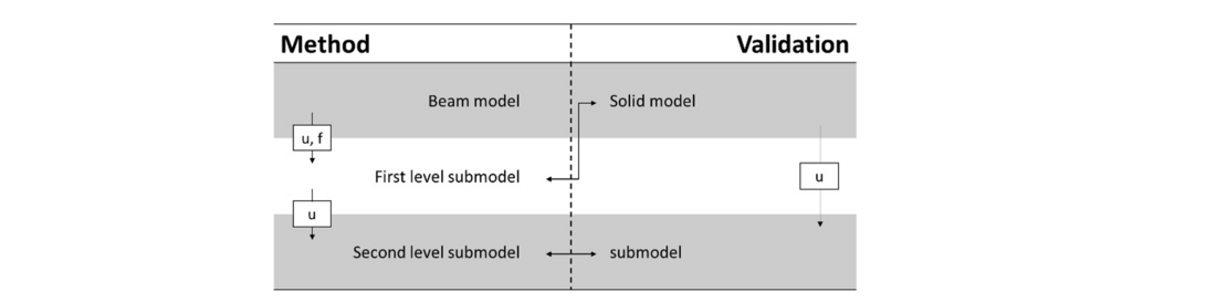
Figure 3 - Multi-scale finite element modelling strategy and validation
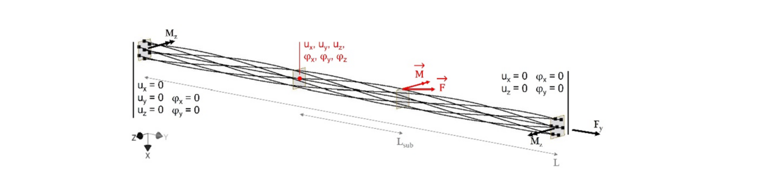
Figure 4 - Beam model used for the presented modelling strategy with its boundary conditions and the boundary conditions transferred to the first level submodel
Investigating a simple, yet relevant loading scenario for overhead line conductors, tension and bending are applied to the global beam model using remote boundary conditions and loads. They are indicated in black. A clamping device is not included to keep the model as simple as possible. All degrees of freedom on one end are set to zero, except for the rotation about the z-axis. On the other end, the rotation about the z-axis and translation along the y-axis are unconstrained. In the first load step (LS1), a tension force Fy is applied on this end. A bending moment Mz about the z-axis on each end is added in the second load step (LS2). The load levels for Fy and Mz given in the following sections are not related to a real load situation.
A solid model of length Lsub represents the first level submodel (see Fig. 5). The boundary conditions which are transferred from the beam model to the solid submodel are indicated in red, exemplary for one wire. For each wire, all six degrees of freedom (three displacements and three rotations) are transferred on the left-hand side using a separate remote displacement object for each wire, that by default is rigid (basically this is done by a multi-point constraint command within the used software). This way, the nodal beam results (displacements and rotations) of the global beam model are translated to displacement boundary conditions acting on the end faces of the wires of the first level submodel. On the right-hand side, the internal reaction loads, namely forces and moments, are transferred for each wire applied to a remote point, that is by default deformable. Subsequently, no additional boundary conditions are necessary in the submodel since the transferred displacements prevent rigid body motion.
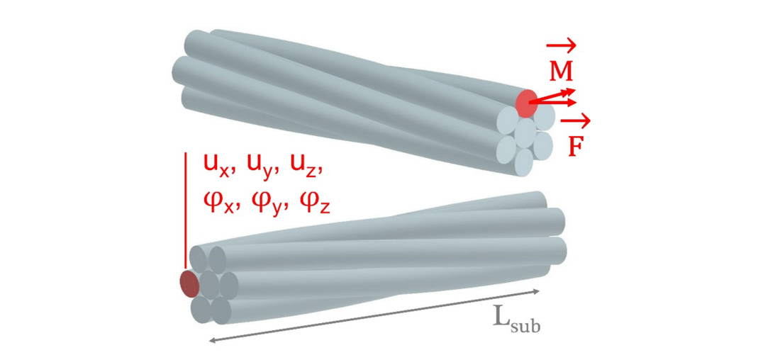
Figure 5 - First level submodel used for the presented modelling strategy with its geometry and boundary conditions
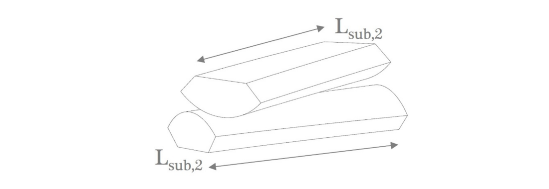
Figure 6 - Second level submodel used for the presented modelling strategy with its geometry
The second level submodel is used for multi-layered cables. According to Fig. 6 two pieces of two crossing wires (length Lsub,2) of the outermost layers are examined in a separate solid model. Since this is a solid-to-solid submodel, only displacements are transferred from the first level submodel to the second level submodel. This is done on all boundaries, where the model is cut.
2.2. Validation
The modelling strategy is validated using a solid model. This solid model has the same geometrical set-up as the global beam model. It validates the first level submodel by results comparison. To validate the local stresses obtained with the second level submodel, this same global solid model is used to extract a solid submodel which has the same dimensions as the second level submodel. The validation approach is shown in Fig. 3. Furthermore, results are compared to the MoCon model [10]. The MoCon model is a beam model developed by Baumann and Novak. It was developed using the properties of an ACSR (Aluminium Conductor Steel Reinforced) Drake conductor. For the validation, its methodology is applied on the geometry which is used in this paper. The MoCon model assumes node-to-node contact at the actual location of the contact between two wires. These contacts allow transferring tangential forces originating from friction effects and leading to a torsional loading of the wires. Standard beam-to-beam contacts, which are used here, are not able to reproduce this behaviour.
2.3. FE Models
All FE models were developed and tested using Ansys Mechanical 2020R2. The studied cables are based on the properties of an ACSR Cardinal conductor. This cable is normally composed of a steel core wire with a surrounding first layer of six wires. This layer is surrounded by three additional layers consisting of 54 aluminium wires. However, to avoid contacts between wires of different material, typical material properties of steel are used for all layers. Otherwise, steel-aluminium and aluminium-aluminium contacts would also be present in the model which would complicate result comparison and interpretation. A linear-elastic material model with a Young’s modulus of E = 210 GPa and a Poisson’s ratio of ν = 0.3 is used. All contacts are frictional with a friction coefficient of μ = 0.5, which is taken from [10]. Circumferential contacts between wires of the same layer are neglected. Solid models are solved using an Augmented Lagrange contact algorithm for line contacts and a Pure Penalty contact algorithm with a normal contact stiffness of 104 N/mm for point contacts. This contact stiffness was found to generate accurate results within reasonable time and was therefore used in this work. Beam models use an Augmented Lagrange contact algorithm. When these parameters differ for a model, it is explicitly mentioned. Solid models are meshed with quadratic hexahedron and tetrahedron elements. Beam models are meshed with linear beam elements (beam elements with 2 nodes and linear interpolation) or quadratic beam elements (beam elements with 3 nodes and quadratic interpolation functions). The beam elements in use are specified for each model. Element size varies between models and is mentioned in the following sections. All simulations were run on a Windows 10 (build: 19041) computer. An Intel(R) Xeon(R) CPU E5-2687W v4 @ 3.00 GHz running on 8 cores with 256 GB available RAM was used.
3. Single-Layer Cable
As a first step, a simple cable composed of a core wire and only one layer of six surrounding strands is studied. The geometrical properties of this single layer cable are shown in Table I. The diameter of the six surrounding strands is reduced because circumferential contact between wires of the same layer is neglected.
Layer | Wires | Wire diameter | Lay angle |
|---|---|---|---|
Core | 1 | 3.34 | - |
1 | 6 | 3.16 | 6.06 |
The length L of the global model is in this case 200 mm. It is relatively short in order to allow a validation with a solid model with reasonable computing cost. The submodelling strategy defined in section 2 is applied. However, only one submodelling step is used because all contacts in this single layer cable are line contacts and not crossing contacts as found for subsequent layers of stranded cables. Therefore, the second submodelling step is not directly applicable in this case. In Fig. 7 to 9 the FE-models of the single-layer cable are shown. The global solid model consists of 3.1 million elements and 13.3 million nodes. The beam model is meshed using 2′800 linear elements of size 0.5 mm. 0.8 million elements and 3.4 million nodes build the mesh of the beam-to-solid submodel, which has a length of 50 mm. This length is necessary to account for boundary condition effects occurring in the model, which will be investigated later in this section. Figure 10 shows the mesh near the contact zones, which was chosen to be identical for the solid model and the beam-to-solid submodel for comparison purposes. Elements in the contact region have a width and depth of 33 μm and a length of 200 μm. The load case presented in section 2 is applied with loads of 5 kN and 10 Nm for tension and bending, respectively.
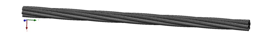
Figure 7 - Single-layer solid FE-model
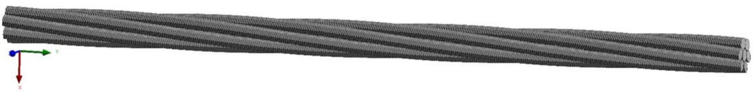
Figure 8 - Single-layer beam FE-model
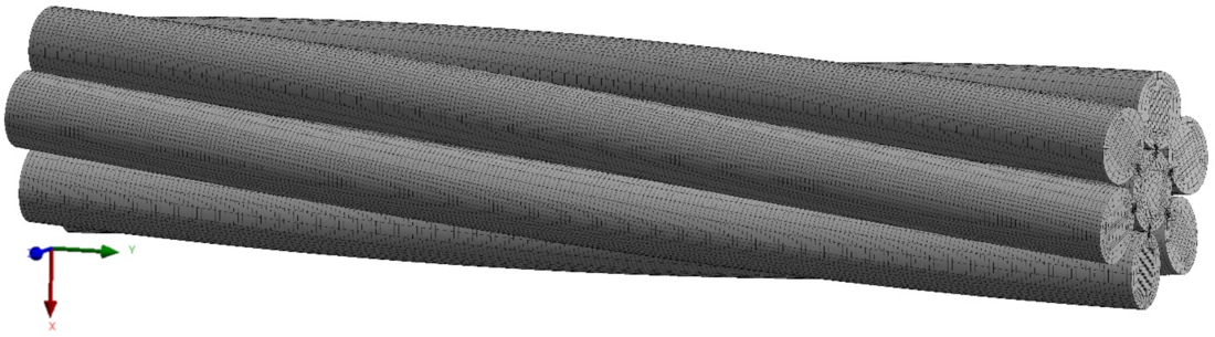
Figure 9 - Single-layer first level FE-submodel
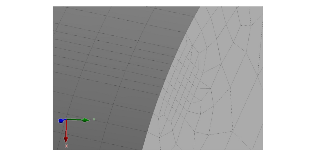
Figure 10 - Detail view of contact mesh in single-layer solid FE-models
Method | ΔL | p | σc,max | σeq,max |
|---|---|---|---|---|
MoCon | 0.0866 | - | - | - |
Solid model | 0.0874 | 2.433 | 72.7 | 123.28 |
Beam model | 0.0867 | 2.430 | - | - |
Submodel | - | 2.445 | 72.1 | 123.04 |
Analytical Solution | 0.0868 | 2.415 | - | - |
The global elongation ΔL is shown to be very similar to the result obtained with the existing MoCon model. The elongation results for the solid and beam FE-models are plotted in Fig. 11. The fact that the scales of the colour maps are almost identical here means that the tensile behaviour of the models is similar.
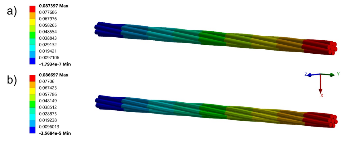
Figure 11 - Plot of elongation results (y-direction [mm]) for single-layer solid (a) and beam (b) FE-models after LS1
The solid model and the beam-to-solid submodel allow evaluating the maximum normal contact pressure σc,max as well as the maximum equivalent von Mises stresses σeq,max in the contact region. In Table II both stress values are almost identical. They occur in the same location in the respective models. Additionally, for a single-layer cable under pure tension analytical solutions exist for the elongation and the length-related radial force p, which is also shown in Table II and can be used for validation. Referencing Feyrer [33], those values can be computed for the given cable by the following equations
(1)
(2)
where (see also Table I) T is the cable tension force, A0 and A1 represent the cross sections of core and first layer wires, d0 and d1 the wire diameters and α the wire lay angle. In Table III, similar results are shown for load step 2.
Method | umax | σeq,max |
|---|---|---|
MoCon | 1.7895 | - |
Solid model | 1.8194 | 254.02 |
Beam model | 1.7395 | - |
Submodel | - | 253.39 |
In this case, it is interesting to compare the maximum transverse deflections umax, which are relatively close between the MoCon model, the beam model and the solid model. The difference between the beam and the solid model is less than 5%. The directional deformation results for the solid and beam FE-models are plotted in Fig. 12. In this figure, the scales of the colour map show that there is a slightly different behaviour.
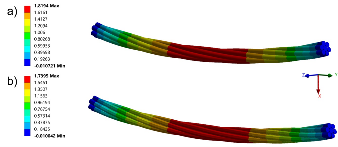
Figure 12 - Plot of deflection results (x-direction [mm]) for single-layer solid (a) and beam (b) FE-models after LS2
The maximum equivalent von Mises stresses obtained with the submodel after load step 2 is only 0.25% lower than the one obtained with the solid model. Maximum stresses occur in the same location in the respective models. Fig. 13 plots the maximum equivalent von Mises stress along the contact zones in the region of interest (ROI) for the solid model and the beam-to-solid submodel for load step 1. The equivalent von Mises stress of the core wire in the submodel is shown in Fig. 14. Fig. 15 plots the maximum equivalent von Mises stress along the contact zone of wire 6 with the core wire in the ROI for load step 2, comparing the solid model and the beam-to-solid submodel. The ROI here corresponds to the submodel region. The stresses on the left-hand side of the submodel where displacements are applied have some divergences compared to the solid model. However, it is seen that at a short distance from the submodel boundary, this error becomes very small.
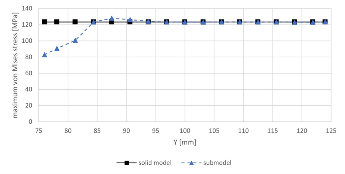
Figure 13 - Diagram comparing the equivalent von Mises stress results in the line contact zone of one wire of the single-layer submodel to the solid model in the ROI after LS1
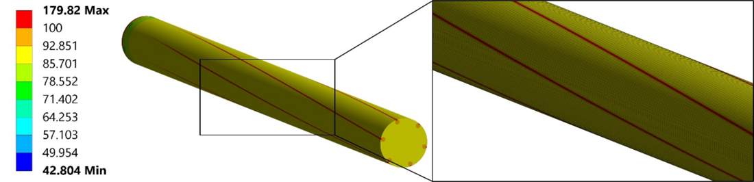
Figure 14 - Plot of the equivalent von Mises stress results in the core wire of the single-layer submodel after LS1
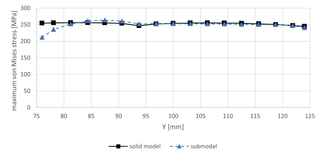
Figure 15 - Diagram comparing the equivalent von Mises stress results in the line contact zone of wire 6 of the single-layer submodel to the solid model in the ROI after LS2
To further study the contact zones in the cable, Fig. 16 shows the maximum contact pressure in the six contact regions between the wires of the first layer and the core wire. It shows only the values in the centre of the ROI and it is verified that these values are representative of this region and that there are no higher values nearby. It is seen that the contact pressure in the submodel is on average 6.2% smaller than in the solid model. This may be due to the transfer of displacements on the left-hand side of the submodel, which was found to create deviations in contact forces and stresses. Although some difference appears in the tension and bending load case for the transverse deflection and the contact pressure, this first model underlines the validity of the proposed strategy for a single-layered cable.
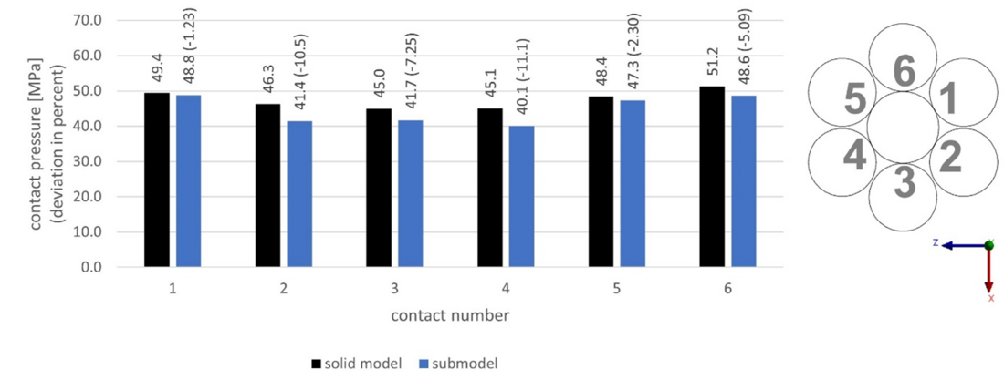
Figure 16 - Diagram comparing contact pressure results of the single-layer submodel to the solid model (middle cross section of ROI after LS2) and cross section view with numbered contacts
4. Two-Layer Cable
To investigate and verify the validity of a local submodel of a beam-to-solid submodel and hence the second step of the modelling strategy explained in section 2, a two-layer cable is modelled. Its geometrical properties are listed in Table IV. Again, here the diameter of the wires in the two layers is reduced because circumferential contact between wires of the same layer is neglected.
Layer | Wires | Wire diameter | Lay angle |
|---|---|---|---|
Core | 1 | 3.34 | - |
1 | 6 | 3.16 | 6.06 |
2 | 12 | 3.16 | 11.99 |
The length of the global model is 200 mm. The solid model that serves for the validation has a contact element size of 0.1 mm (6.5 million elements and 16.9 million nodes). In Fig. 17, three differently meshed beam models are shown.
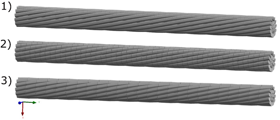
Figure 17 - Two-layer beam FE-models 1, 2 and 3 with different discretization
These three models will be used to investigate the sensitivity of the results to the beam discretization and type of beam elements. Models 1 to 3 have a beam element size of 1 mm (3′800 linear beam elements), 4 mm (950 quadratic beam elements) and 8 mm (475 quadratic beam elements). The beam-to-solid submodel, which has an overall length of 50 mm (1.5 million elements and 3.9 million nodes) is shown in Fig. 18. The contact zones between the first and second layer have a refined mesh (see Fig. 18, b) with minimum element size of 0.1 mm, which is identical to the one in the solid model used for validation.
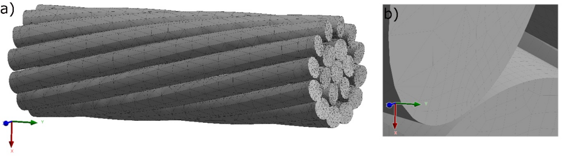
Figure 18 - Two-layer FE first level submodel (a) and detail view of its contact mesh (b)
Fig. 19 shows the mesh of the local submodel, which is extracted from the beam-to-solid submodel, in the region of a contact in the outer two layers. The element size in the contact zone is 5 μm and the size of each wire section is 0.83 mm in radial direction and 2.234 mm at the widest position. It consists of 0.6 million elements and 1.7 million nodes. The local submodel extracted from the solid model for validation has the same size and mesh properties. The load applied to the global models is composed of 13.5 kN in tension and 27 Nm bending.
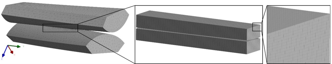
Figure 19 - Two-layer second level submodel
The total computation time used for the submodelling process is less than 10 h (beam model 0.25 h, first level submodel 7.75 h, second level submodel 1.25 h) on the hardware mentioned in section 2.3. In comparison, the solid model used for validation had a computation time of about 31 h for a mesh refinement level equivalent to the first level submodel mesh, but 20 times coarser than in the second level submodel contact zone. Those numbers underline the efficiency of the presented approach and give proof of the fact that for an equivalent level of meshing for a solid model, the computation time would not be practical.
Table V lists the elongation for load step 1 and the transverse deflection for load step 2 and compares them to the results obtained with the MoCon model and the solid model. It can be seen that the elongation in tension is similar for all models with a difference of less than 4%. Also, this result is not sensitive to the discretization of the beam model. However, the deflection obtained with the beam model is shown to be very sensitive to the beam discretization and very different from the MoCon and solid models in the case of beam model 1 and 3. This unexpected bending behaviour may be due to different contact states and distribution of contact forces within the models.
Method | ΔL | umax |
|---|---|---|
MoCon | 0.0918 | 1.44 |
Solid model | 0.0951 | 1.45 |
Beam model 1 | 0.0922 | 1.14 |
Beam model 2 | 0.0926 | 1.43 |
Beam model 3 | 0.0925 | 1.75 |
Method | σc,max,LS1 | σeq,max,LS1 | σc,max,LS2 | σeq,max,LS2 |
|---|---|---|---|---|
Local submodel solid | 2537.8 | 1479.6 | 2520.8 | 2485.2 |
Local submodel beam 1 | 2561.2 (+0.92) | 1491.5 (+0.80) | 2529.2 (+0.33) | 2772.8 (+11.6) |
Local submodel beam 2 | 2553.4 (+0.61) | 1487.5 (+0.53) | 2533.5 (+0.50) | 2546.7 (+2.47) |
Local submodel beam 3 | 2544.5 (+0.26) | 1483.4 (+0.26) | 2537.9 (+0.68) | 2544.9 (+2.40) |
On the other hand, as shown in Table VI, the maximum contact pressure σc,max and maximum equivalent von Mises stress σeq,max in the different local submodels are in general very close for both load steps. The only important difference occurs for the local submodel originating from beam model 1, which has a difference of 11.6% to the validation local submodel. Stresses are evaluated exclusively in the local submodels. The mesh of the submodels does not allow a stress evaluation with the required accuracy for a comparison between the two. To further investigate the differences obtained, the forces at one contact are extracted for the different models and submodels for load step 1 (Fig. 20) and load step 2 (Fig. 21).
Fig. 20 shows that these contact forces are very similar between the various models. However, in Fig. 21, where the contact forces at contact 1 are again shown for the various models and submodels after load step 2, it is clear that the variation is more pronounced when bending is applied and reaches 11.1% in the case of beam model 3.
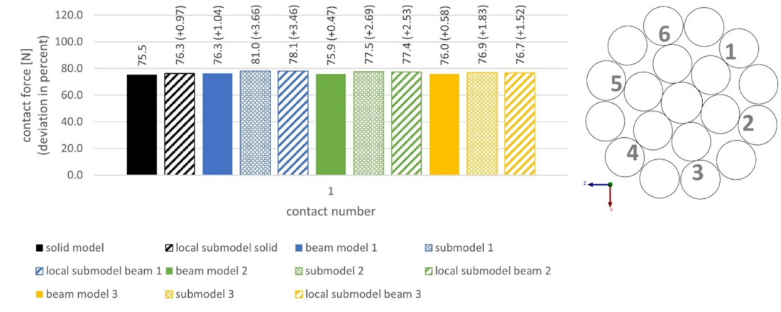
Figure 20 - Diagram comparing contact force results of all two-layer FE-models for contact 1 (near middle cross section of ROI after LS1) and cross section view with numbered contacts
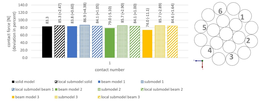
Figure 21 - Diagram comparing contact force results of all two-layer FE-models for contact 1 (near middle cross section of ROI after LS2) and cross section view with numbered contacts
Fig. 22, which shows the contact forces at all six contact points identified in Fig. 21, confirms that the global beam models have a distribution of contact forces within the wires that is significantly different from the solid models and submodels when bending is applied. However, when transferring the boundary conditions to the beam-to-solid submodel and then to the local submodel, the differences in terms of contact pressure and local equivalent von Mises stresses in the contact regions become relatively small. This is confirmed in Fig. 23, where the distribution of equivalent von Mises stresses after load step 2 is shown to be very similar between the different local submodels. Overall, the bending behaviour seems to be sensitive to the type and length of beam element used. This should be further investigated to understand this effect, especially if the model needs to be used to evaluate the deformed shape of cables. However, for the purpose of this study, the stress at the contact was not found to be sensitive to this parameter, and therefore, the length and type of beam element can be selected according to the size and computation time of the models as it will be done in the four-layer cable in Section 5.
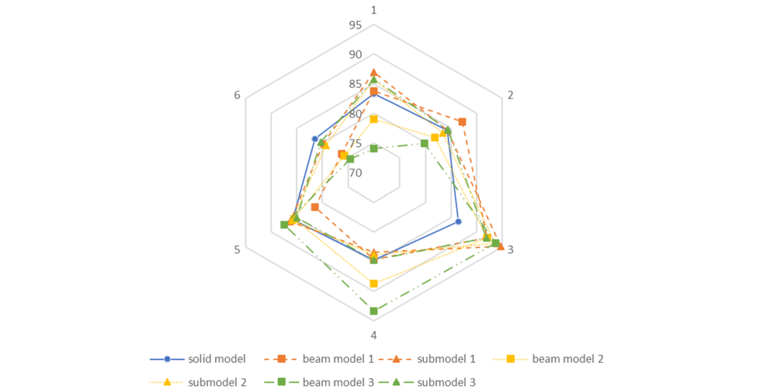
Figure 22 - Diagram comparing contact force results for the two-layer solid, beam and first level submodel for contacts 1 to 6 (near middle cross section of ROI after LS2)
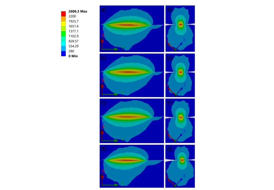
Figure 23 - Plot of equivalent von Mises stress results of the following two-layer FE-models (in MPa, after LS2, two cross section views of each model): submodel level 2 validation (a), submodel level 2 of beam 1 (b), beam 2 (c) and beam 3 (d)
5. Four-Layer Cable
Finally, the developed finite element beam-to-solid submodelling strategy is applied to a four-layer cable, which represents a practically relevant wire or cable like conductor. Its geometrical properties are listed in Table VII. Here, the actual diameters of the cables were modelled in order to geometrically represent a relevant cable. However, circumferential contact between wires of the same layer is still neglected.
Layer | Wires | Wire diameter | Lay angle |
|---|---|---|---|
Core | 1 | 3.34 | - |
1 | 6 | 3.34 | 6.06 |
2 | 12 | 3.32 | 11.99 |
3 | 18 | 3.32 | 11.8 |
4 | 24 | 3.32 | 13.10 |
Fig. 24 shows the mesh of the different FE-models. The boundary effects are more pronounced in the case of a four-layer cable. To avoid boundary effects near the submodel region, this model is longer compared to the single-layer and two-layer cables and has a length of 400 mm. In order to keep reasonable computation times, the mesh of the solid model used for validation is coarser than the corresponding model in section 4. It has 1.2 million elements and 5.2 million nodes and a contact element size of 0.5 mm (width and depth) times 1 mm (length). The beam model is meshed with 11′500 linear elements. It uses element sizes of 8 mm (core), 4 mm (first layer) and 2 mm (second, third and fourth layer). The beam-to-solid submodel, which has an overall length of 50 mm (4 million elements and 10.4 million nodes) is shown in Fig. 24c. The wire-to-wire contact zones between layers have a refined mesh with minimum element size of 0.1 mm. The mesh of the local submodel has approximately the same properties as the model shown in Fig. 19 and used in section 4 (0.6 million elements and 1.7 million nodes). In this case, a submodel could not be extracted from the validation solid model because of its coarse mesh. The tension force and bending moments applied are 40 kN and 80 Nm, respectively.
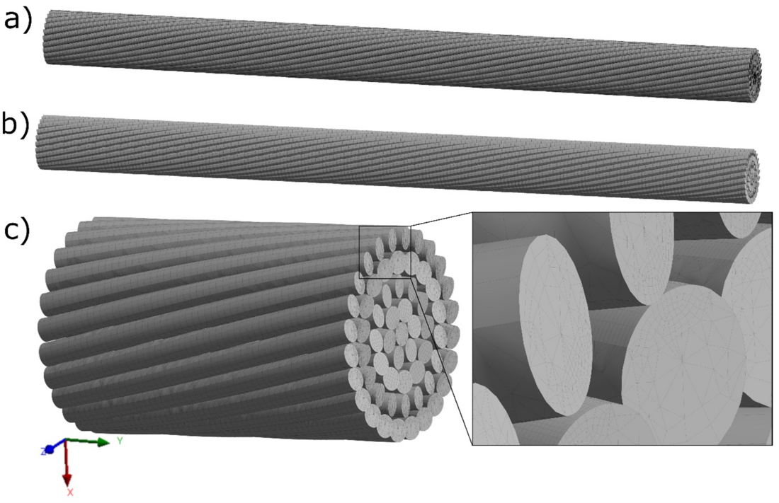
Figure 24 - Four-layer FE solid model (a), beam model (b) and submodel level 1 with detail view of its contact mesh (c)
The total computation time used for the submodelling process is less than 33 h on the hardware mentioned in section 2.3. The major part, 29 h, is used for the first level submodel. In comparison, the solid model used for validation, which has a much coarser mesh, had a computation time of about 8.5 h. Detailed computation times are shown in Table VIII.
Method | Computation time |
|---|---|
Solid model | 8.5 |
Beam model | 2.3 |
Submodel | 29.3 |
Local submodel | 1.0 |
Method | ΔL | umax |
|---|---|---|
MoCon | 0.1711 | 1.11 |
Solid model | 0.1832 | 1.31 |
Beam model | 0.1686 | 1.14 |
Table IX presents the elongation results for load step 1 and the bending deflection for load step 2. This time the difference in elongation between the solid model and beam model is slightly higher (8%), while the difference between the MoCon model and beam model remains relatively low (1.5%). Again, important differences are observed between the solid and beam model, but this time the result of the transverse deflection of the beam model is very close to the MoCon model for the selected mesh. Average contact force results for the contacts occurring between wires of the fourth and third layer in different longitudinal positions (Y coordinates) in the ROI are given in Table X and Fig. 25 for load step 1.
Y | Solid model | Beam model | Submodel | Deviation |
|---|---|---|---|---|
197.74 | 30.64 | 39.95 | 33.00 | +7.73 |
200.01 | 17.52 | 20.37 | 14.00 | -20.1 |
202.28 | 20.84 | 26.44 | 23.95 | +14.9 |
204.55 | 30.62 | 34.09 | 30.69 | +0.24 |
206.83 | 14.92 | 7.99 | 14.98 | +0.37 |
209.10 | 26.77 | 31.04 | 28.21 | +5.37 |
211.37 | 28.86 | 28.11 | 30.10 | +4.28 |
213.65 | 17.12 | 8.89 | 16.06 | -6.18 |
215.92 | 28.37 | 36.35 | 28.30 | -0.26 |
218.19 | 22.30 | 23.40 | 25.88 | +16.0 |
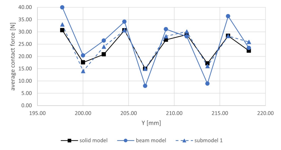
Figure 25 - Diagram comparing average contact force results of the four-layer solid model, beam model and first level submodel (ROI after LS1)
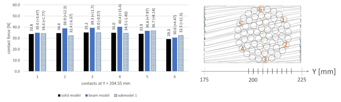
Figure 26 - Diagram comparing contact force results of the four-layer solid model, beam model and first level submodel in contacts 1 to 6 (near middle cross section of ROI after LS2) and cross section view with numbered contacts
Some scatter between the different models is observed (up to 20.1%), but they tend to decline as we approach the centre of the ROI. In Fig. 26, the contact forces at six locations between the last two layers are shown. These forces are in the same range even if the mesh refinement and model size are very different. To further exploit the capacity of the submodelling strategy, the equivalent von Mises stresses in one contact region, again between the outer two layers, were extracted from the local submodel. They are presented in Fig. 27 and show well the specific behaviour of the contact zone when combined tension and bending loads are applied. Fig. 28 shows the contact pressure distribution and the contact status for load step 2. This level of modelling, which can represent the detailed stresses at and around the contact zones, is the one needed when assessing the fatigue behaviour of cables under complex loading.
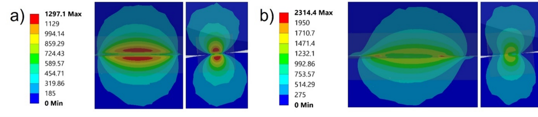
Figure 27 - Plot of equivalent von Mises stress results of the four-layer second level submodel after LS1 (a) and after LS2 (b) given in MPa
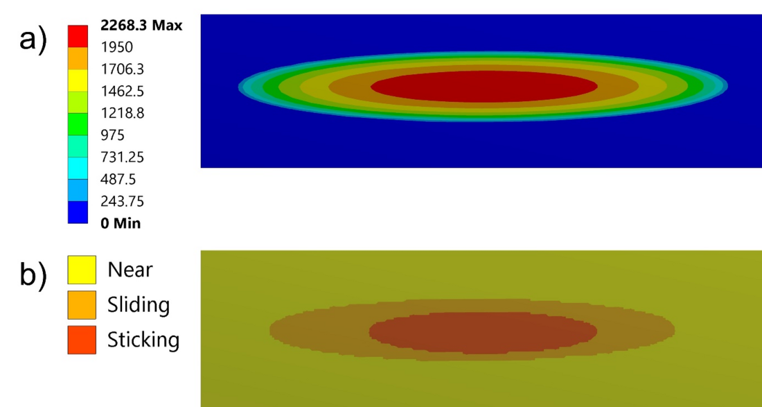
Figure 28 - Plot of contact pressure results in MPa (a) and contact status (b) of the four-layer second level submodel after LS2
6. Conclusion
A multi-scale finite element strategy was developed to compute the stresses in the vicinity of the contact zones between crossing wires of the two outermost layers of a stranded cable and presented in this paper. The strategy is based on a global beam model with contacts subject to both tension and bending loads and includes two submodelling steps to obtain a very refined local submodel in which stresses at and around contact zones can be evaluated precisely. The following conclusions were drawn from this study:
- The first submodelling step, consisting of applying a combination of forces and displacements extracted from the beam model on individual wires of a solid submodel has shown to provide good results when compared to a refined solid model in the case of a single-layer cable.
- The first submodelling step requires a solid model including the whole cable cross section in order to correctly import the boundary conditions from the global beam model. A certain submodel length is needed to account for the boundary effects. This length is independent of the total length of the global beam model.
- Analyses on a two-layer cable showed that the results of deflection under bending load are sensitive to the beam discretization. Furthermore, beam models show some differences in terms of contact forces compared to the first or second level submodels. However, when transferring the boundary conditions to the local submodels, the differences in terms of contact pressure and equivalent von Mises stress become very small. The impact of the possible inaccuracies of the beam model therefore appears to be negligible in the overall submodelling strategy.
- The methodology could also be applied to a four-layer cable, which highlighted the potential of the strategy to evaluate detailed stresses at the contact level of stranded cables such as conductors.
The developed method is hence a valid approach to solve the complex problem of studying detailed stresses causing fatigue at the contact level while keeping realistic loading conditions of a cable subjected to tension and bending. In the next steps, the clamping device and the aluminium material of the outer layers could be modelled in the global model in order to study realistic conditions found in overhead line conductors. This step increases significantly the complexity of the global model, but can be achieved as shown in the work of Lalonde et al. [9]. This approach could then be integrated in numerical tools for the evaluation of the fatigue life of conductors. Again, this step asks for an important adaptation of existing methods of fretting-fatigue evaluation and a thorough validation with experimental data at the contact and the conductor-clamp scales. Those steps would lead to an advanced but practical tool for evaluating the fatigue life of various overhead line clamp and conductor configurations.
References
- P. H. C. Rocha, J. I. M. Díaz, J. A. Araújo, F. C. Castro, “Fatigue of two contacting wires of the ACSR Ibis 397.5 MCM conductor. Experiments and life prediction,” International Journal of Fatigue, vol. 127, pp. 25-35, Oct. 2019.
- I. M. Matos, P. H. C. Rocha, R. B. Kalombo, L. A. C. M. Veloso, J. A. Araújo, F. C. Castro, “Fretting fatigue of 6201 aluminium alloy wires of overhead conductors,” International Journal of Fatigue, vol. 141, Dec 2020.
- K. O. Papailiou, “On the bending stiffness of transmission line conductors,” IEEE Transactions on Power Delivery, vol. 12, Oct. 1997.
- J. C. Poffenberger, R. L. Swart, “Differential displacement and dynamic conductor strain,” IEEE Transactions on Power Apparatus and Systems, vol. 84, Apr. 1965.
- A. A. Fadel, D. Rosa, L. B. Murça, J. L. A. Ferreira, J. A. Araújo, “Effect of high mean tensile stress on the fretting fatigue life of an Ibis steel reinforced aluminium conductor,” International Journal of Fatigue, vol. 42, pp. 24-34, Sep. 2012.
- J. Chan, C. Rawlins, G. Diana, L. Cloutier, J.-L. Lilien, C. Hardy, EPRI Transmission line reference book: Wind-induced conductor motion (1012317), EPRI, 2006.
- C. R. F. Azevedo, A. M. D. Henriques, A. R. Pulino Filho, J. L. A. Ferreira, J. A. Araújo, “Fretting fatigue in overhead conductors. rig design and failure analysis of a Grosbeak aluminium cable steel reinforced conductor,” Engineering Failure Analysis, vol. 16, pp. 136-151, Jan 2009.
- F. Levesque, S. Goudreau, A. Cardou, L. Cloutier, “Strain measurements on ACSR conductors during fatigue tests I - experimental method and data,” IEEE Transactions on Power Delivery, vol. 25, Oct. 2010.
- S. Lalonde, R. Guilbault, F. Légeron, “Modeling multilayered wire strands, a strategy based on 3D finite element beam-to-beam contacts - part I: Model formulation and validation,” International Journal of Mechanical Sciences, vol. 126, pp. 281-296, Jun. 2017.
- R. Baumann, P. Novak, “Efficient computation and experimental validation of ACSR overhead line conductors under tension and bending,” CIGRE Science & Engineering, vol. 9, pp. 5-16, Oct. 2017.
- A. Naworocki, M. Labrosse, T. Conway, A new specific finite element model for cables - part I: Theory, Wire Journal International (2000).
- R. Beleznai, I. Páczelt, “Design curve determination for two-layered wire rope strand using p-version finite element code,” Engineering with Computers, vol. 29, pp. 273-285, Jul 2012.
- W. Zhou, H. Q. Tian, “A novel finite element model for single-layered wire strand,” Journal of Central South University, vol. 20, pp. 1767-1771, Jun 2013.
- V. Ivanco, S. Kmet, G. Fedorko, “Finite element simulaiton of creep of spiral strands,” Engineering Structures, vol. 117, pp. 220-238, Jun 2016.
- J. Said, S. Garcin, S. Fouvry, G. Cailletaud, C. Yang, F. Hafid, “A multi-scale strategy to predict fretting fatigue endurance of overhead conductors,” Tribology International, vol. 143, Mar 2020.
- K. Schillai, “Enhanced fretting fatigue resistance of conductors for high voltage overhead lines,” Ph.D. dissertation, ETH Zurich, 2019.
- S. R. Ghoreishi, T. Messager, P. Cartraud, P. Davies, “Validity and limitations of linear analytical models for steel wire strands under axial loading, using a 3D FE model,” International Journal of Mechanical Sciences, vol. 49, pp. 1251-1261, Nov. 2007.
- E. Stanova, G. Fedorko, M. Fabian, S. Kmet, “Computer modelling of wire strands and ropes part I: Theory and computer implementation,” Advances in Engineering Software, vol. 42, pp. 305-315, Jun 2011.
- R. Judge, Z. Yang, S. W. Jones, G. Beattie, “Full 3D finite element modelling of spiral strand cables,” Construction and Building Materials, vol. 35, pp. 452-459, Oct 2012.
- W. G. Jiang, “A concise finite element model for pure bending analysis of simple wire strand,” International Journal of Mechanical Sciences, vol. 54, pp. 69-73, Jan 2012.
- M. Frigerio, P. B. Buehlmann, J. Buchheim, S. R. Holdsworth, S. Dinser, C. M. Franck, “Analysis of the tensile response of a stranded conductor using a 3D finite element model,” International Journal of Mechanical Sciences, vol. 106, pp. 176-183, Feb. 2016.
- G. Qi, Computational modeling for stress analysis of overhead transmission line stranded conductors under design and fretting fatigue conditions, Ph.D. dissertation, Department of Civil Engineering and Applied Mechanics, McGill University, Montreal, Apr. 2013.
- A. Cruzado, S. B. Leen, M. A. Urchegui, X. Gómez, “Finite element simulation of fretting wear and fatigue in thin steel wires,” International Journal of Fatigue, vol. 55, pp. 7-21, Oct. 2013.
- F. Lévesque, S. Goudreau, L. Cloutier, “Elastic-plastic microcontact model for elliptical contact areas and its application to a treillis point in overhead electrical conductors,” Journal of Tribology, vol. 133, Jan. 2011.
- C. Curreli, M. Viceconti, F. Di Puccio, “Submodeling in wear predictive finite element models with multipoint contacts,” International Journal for Numerical Methods in Engineering, vol. 122, pp. 3812-3823, Aug. 2021.
- C. Curreli, F. Di Puccio, L. Mattei, “Application of the finite element submodeling technique in a single point contact and wear problem,” International Journal for Numerical Methods in Engineering, vol. 116, pp. 708-722, Dec. 2018.
- H. Soo Kim, S. Mall, A. Ghoshal, “Two-dimensional and three-dimensional finite element analysis of finite contact width on fretting fatigue,” Materials Transactions, vol. 52, 2011.
- S. Shankar, R. Nithyaprakash, G. Abbas, R. Naveen Kumar, A. Pramanik, A. K. Basak, “Invitro tribological study and submodeling finite element technique in analyzing wear of zirconia toughened alumina against alumina with bio-lubricants for hip implants,” Medical Engineering and Physics, vol. 98, pp. 83-90, Dec 2021.
- R. Rajasekaran, D. Nowell, “On the finite element analysis of contacting bodies using submodelling,” Journal of Strain Analysis for Engineering Design, vol. 40, Feb. 2005.
- W. J. Elke III, M. W. Sracic, “Effects of cut boundary location on finite element submodels with contacts,” in Proc. ASME 2019 International Design Engineering Technical Conferences.
- N. G. Cormier, S. B. S., G. B. Sinclair, G. Meda, “Aggressive submodelling of stress concentrations,” International Journal of Numerical Methods in Engineering, vol. 46, pp. 889-909, Oct. 1999.
- F. Lanoue, A. Vadean, B. Sanschagrin, “Finite element analysis and contact modelling considerations of interference fits for fretting fatigue strength calculations,” Simulation Modelling Practice and Theory, vol. 17, pp. 1587-1602, Nov 2009.
- K. Feyrer, Wire Ropes, Springer Berlin, Heidelberg, 2015.
Biographies
Sascha Jabornegg finished his master studies at Lucerne University of Applied Sciences and Arts in 2021, following his bachelor’s degree in mechanical engineering. In his master’s thesis, he focussed on the application of the Finite Element Method on multi-layered wire strands using Ansys Workbench. Currently, Sascha Jabornegg is employed by EnDes Engineering Partner AG as a development engineer.
Ralf Baumann studied Aerospace Engineering at the University of Stuttgart and graduated as Dipl.-Ing. in 1992. His employment experience includes several research and management positions at Hilti AG, Principality of Liechtenstein. In 2005 he moved to Lucerne University of Applied Sciences and Arts, Department Mechanical Engineering, as a lecturer for the Finite Element Method and Lightweight Structures. Since 2006 he is Head of the Competence Centre Mechanical Systems and received the professorship in 2007. His research activities comprise the field of computational mechanics and cables.
Sébastien Langlois has received his Ph.D. from Université de Sherbrooke, Canada in 2013 and his B. Eng. and M. Eng. in civil engineering from McGill University, Canada in 2005 and 2007 respectively. He is a registered professional engineer in the province of Québec, Canada. Since 2014, he is a professor in the civil and building engineering department at Université de Sherbrooke. His main research interests are the behaviour of transmission line towers, the evaluation of conductor oscillations and damages, and the effect of wind on structures.
Pedro Henrique Rocha is a PhD. student at Université de Sherbrooke. He received his BSc. in Mechanical Engineering and MSc. in Science Mechanics from University of Brasília in 2016 and 2019, respectively. Pedro Henrique carries out research about the fatigue behaviour of overhead conductors and aluminium wires subjected to fretting fatigue conditions since 2015. Over the years, he authored and co-authored more than 10 scientific papers in international journals and conferences. Currently, his PhD. research concerns the proposition of life estimation methods for overhead conductors based on the similitude with fretting fatigue tests on wires.