Day-ahead prediction of short-term voltage drops by random forest method
Authors
L. VAN ALTENA, S. STEIN, S. DOROUDIAN, DR. T. RINGELBAND - Amprion GmbH
DR. S. KIPPELT - EF. Ruhr GmbH

Summary
The European Transmission System is undergoing a transformation as many fast-acting electrical devices are integrated into the system on generation, load and grid side, e.g. wind power plants or HVDC systems. The integration of these devices results in faster and steeper gradients of the state variables such as voltage and frequency. Accordingly, short-term voltage drops of high magnitude have been observed more frequently in the recent past. Since such voltage drops can jeopardize secure grid operation, the need to implement a forecasting process that predicts voltage drops day-ahead was identified by the German Transmission System Operators. Within this paper, the development and implementation of the German operational forecast process for short-term voltage drops is presented. In this context, the selection and parameterization of applicable machine learning methods for this process are described. This paper also presents the application and the monitoring of the operational process and evaluates the forecast quality.
Keywords
forecast, German transmission grid operation, machine learning, random forest, voltage dropsNomenclature
aFRR Automatic frequency restoration reserve
AT Austria
CH Switzerland
DK Denmark
MSCDN Mechanically switched capacitor with damping network
OPL Operational Planning
PV Photovoltaic
STATCOM Static synchronous compensator
SVM Support Vector Machine
TSO Transmission system operator
U Voltage
1. Introduction
The reactive power demand of the German transmission grid is constantly increasing due to higher line loadings and expansion of the transmission system. Within their network expansion planning, the German transmission system operators (TSOs) calculated a minimum requirement for stationary and actively controllable reactive power compensation in a magnitude of more than 20 GVAr [1]. While planning and construction of these devices has commenced, challenging voltage phenomena can already be observed today. One of these phenomena are short-term voltage drops, which have been observed repeatedly in the German transmission grid during winter months since 2017. When these voltage drops occur, grid voltage drops by up to 15 kV in several substations within 5 to 10 minutes.
Figure 1 shows the voltage profile of a substation in the north of Germany on 29 January 2018. On this day, the largest voltage drop observed so far took place at 6 a.m.
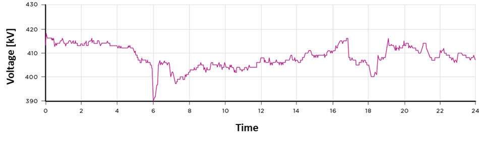
Figure 1 - Voltage profile of a substation in the north of Germany on 29 January 2018
As shown in Figure 2, the voltage drop did not remain local but occurred in many substations covering a large area from the North-East of North Rhine-Westphalia over Hesse and Thuringia up to the North of Bavaria.
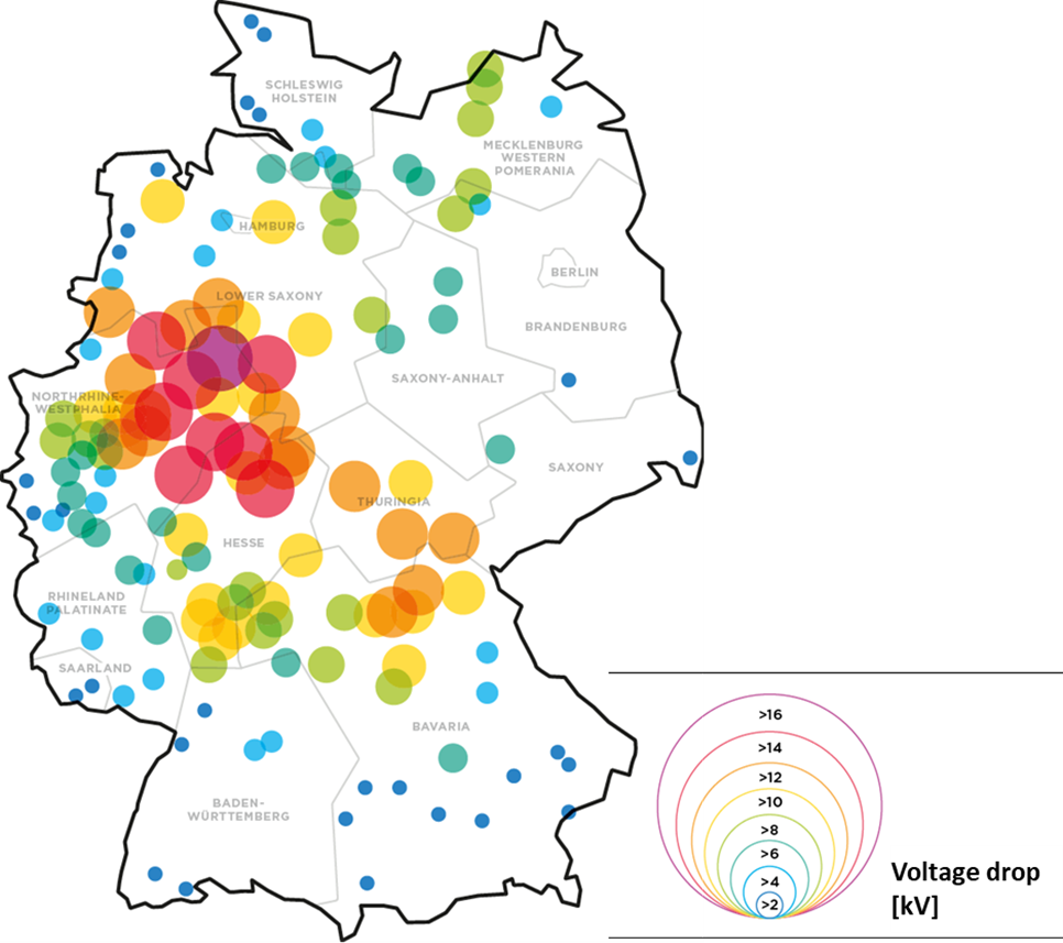
Figure 2 - Regional occurrence of the voltage drops on 29 January 2018
Afterwards, the causes of this voltage drop were investigated in detail. The investigations showed a sudden increase in the voltage angle difference between the north and south of Germany around 6 a.m., increasing the already existing north-south power flows by approximately 1 GW. The resulting additional reactive power demand of the lines could not be compensated due to the low number of conventional power plants in the affected area, leading to voltage drops in several substations located on the transit path. As the main driver for the sudden additional power flow, power infeed characteristics of wind power plants at 6 a.m. were identified. According to [2], certain noise immission guide values may not be exceeded outside of buildings. The regulation distinguishes between daytime and nighttime immission guide values as well as the place of immission (industrial area, commercial area, residential area, etc.). Since the night immission guide values are up to 18 dB below the day immission guide values, depending on the immission location, many wind turbines are forced to switch to noise-reduced operation from 10 p.m. to 6 a.m. and thus to reduce their feed-in power. From 6 a.m. (in some cases staggered from 7 a.m.), the turbines can again feed into the grid at full capacity. Therefore, steep power gradients in the north of the German grid can be observed at 6 a.m., as many wind farms are connected to this grid area via fast acting converters. This effect was increased even further by the commissioning of a new wind farm shortly before 29 January 2018. The power imbalance caused by the fast acting converters was compensated by the use of automatic frequency restoration reserve (aFRR) in the south of Germany, resulting in the additional north-south transit.
In addition to the voltage drop on 29 January 2018, voltage drops with different magnitudes and spatial expansion could be observed more frequently in recent years. Since such voltage drops can jeopardize compliance with the operating voltage range [3] and thus secure grid operation, the need to implement a forecasting process that predicts voltage drops day-ahead was identified by the German Transmission System Operators. Based on such a forecast process, operators can be warned of voltage drops that might cause voltage collapses and plan and evaluate countermeasures against voltage drops in advance.
Thus, initial analyses and the development of an initial forecast method were carried out within a study in 2019 by ef.Ruhr GmbH, a Dortmund-based consultancy [4]. Subsequently, extensive further analyses and significant further developments of forecasting methods were carried out by Amprion GmbH, one of the German TSOs, to date. Chapter 2 summarizes the results of the big data analyses regarding voltage drops using the most current data. In Chapter 3, the selection of the machine learning algorithm which is used for the forecast is presented. In this context, the requirements of a practical forecast method are described and a comparison between potential machine learning algorithms is carried out. As Amprion GmbH implemented an operational forecast process to predict voltage drops for the German Transmission System operators in 2020, the design and application of this process are described in Chapter 4. The continuous monitoring and further developments of this operational process, which are required due to the constant changes in the German Transmission Grid, are presented in Chapter 5. Finally, a conclusion is presented in Chapter 6.
2. Analysis of voltage drops
In order to implement a forecasting process, comprehensive analyses on the occurrence of voltage drops are required. Therefore, Chapter 2.1 gives a brief definition of voltage drops that are to be considered for the forecast. In Chapter 2.2, analyses of the spatial and temporal characteristics of those voltage drops are described in detail. In Chapter 2.3, statistical analyses on causes of voltage drops are presented. In this context, the challenges of analysing big data are highlighted.
2.1. Definition of voltage events
Voltage magnitudes in the substations of the German Transmission System are constantly changing over time due to various factors. In order to predict short-term voltage drops, it is necessary to specify the voltage drops that are to be considered for the forecast regarding a threshold value, a timeframe and the factors that are causing the voltage drops.
According to [3], voltage changes higher than 2 % within 10 minutes should be avoided by German Transmission System Operators. Applying the lower limit of the operating voltage range (390 kV), this results in a threshold value of 7.8 kV that should not be exceeded within 10 minutes.
The main factor for voltage changes is the constant change in active power demand and supply of grid users and the resulting change in the active power flow. Next to those voltage changes caused by active power flow changes, voltage changes can also result by switching operations or the use of reactive power compensation systems. In particular, the operation of MSCDNs and reactors can cause voltage gradients that are very similar to the gradients caused by active power flow changes of wind power plants, which are shown in Figure 1. As switching operations and the use of reactive power systems are executed by the control centers of the German Transmission Operators with the aim to optimize the current grid state, it is not necessary to predict voltage changes caused by these actions. Thus, only voltage drops caused by changes in active power demand and supply resulting in a change of active power flow are to be considered further.
Based on these explanations, voltage drops that are further considered for analyses and the forecast are voltage drops that exceed the threshold value of 7.8 kV withing 10 minutes and are caused by fast active power flow changes. Those voltage drops are referred to as voltage events in the following. Applying this definition, a total of 262 voltage events could be identified in the period from 2017 to 2022 by an identification method, which is presented in Chapter 5.1. It should be noted that fast transient voltage drops are by definition outside the scope of this paper and are therefore not considered for analyses and the forecast presented in the following chapters.
2.2. Spatial and temporal analysis of voltage events
Firstly, voltage events were analysed by their spatial occurrence. Based on these analyses, two regions A and B were identified, with events occurring either in region A or in region B or in both regions simultaneously. In total, region A accounted for 22 % and region B for 40 % of the events, while 38 % of the events occurred in both regions simultaneously (see Figure 3).
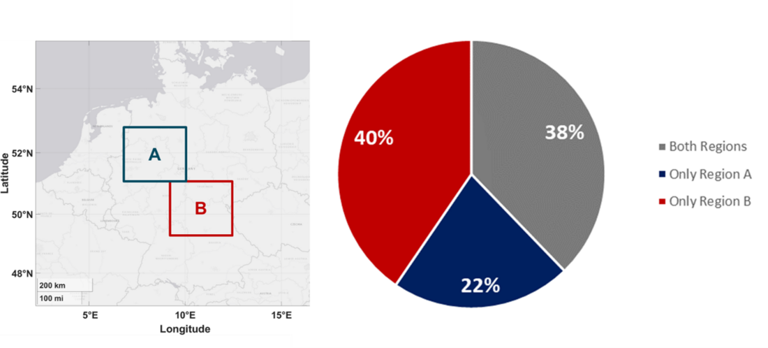
Figure 3 - Spatial classification of regions affected by voltage events (left) and relative proportion of regional occurrence of voltage events (right) in winters 2017/18 - 2021/22
Moreover, voltage events were analysed regarding their temporal occurrence. The analyses showed that more than 60 % of the events occurred at the change of hours at 6 a.m. or 7 a.m. (see Figure 4). For the remaining hours of the day, no particular pattern could be detected.
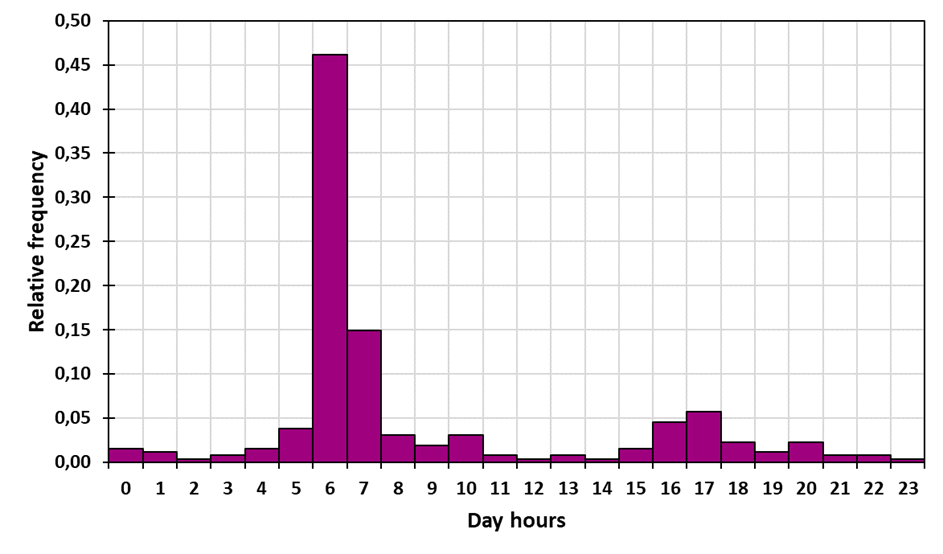
Figure 4 - Relative frequency of the hourly occurrence of the voltage drops in the winters 2017/18 - 2021/22
An evaluation of the average daily voltage curve at selected substations in regions A and B confirms that the voltage drop at 6 a.m. is a common phenomenon (see Figure 5). Between 06:00 and 06:10, a significant voltage drop occurs in large parts of the grid on average over all days studied in 2017/2018, reaching values up to 4.5 kV for a specific substation. Observed voltage events with values greater than 7.8 kV could therefore also be interpreted as noticeable expressions of a usual phenomenon.

Figure 5 - Average daily voltage curve of selected substations in regions A and B
2.3. Root cause analysis of voltage events
In order to identify the causes of the voltage events, statistical analyses of different grid characteristics and the occurrence of voltage drops were carried out. Thus, data of voltages, currents, active and reactive power flows of substations, lines, transformers, power plants and reactive power compensation systems were collected, leading to a total of around 4,000 data points. Depending on the data source and the focus of the analyses, data were analysed at a resolution of 3 seconds to 15 minutes over a period of time ranging from half a year to several years. The resulting data volume of more than 5 billion measured values, as well as the multicollinearity of the data sources among each other, posed a particular challenge for the big data analyses. For a more efficient data handling, only data points that were suspected to be related to the observed phenomenon of voltage drops were examined. These data points included in particular:
- Total vertical grid load of each German TSO
- Power flows on selected lines and corridors
- Dispatch of power plants in regions A and B
- Offshore and onshore wind power feed-in
- Photovoltaic power feed-in
- Use of automatic frequency restoration reserve (aFRR) in each German control area
- Control area program of each German TSO
- Control area demand of each German TSO
- Total grid losses of each German TSO
- Temperatures at different substations
- Day-ahead spot market prices
Various statistical analyses were carried out based on these data points. In this paper, a correlation analysis aiming at investigating the high number of voltage events around 6 a.m. is presented as an example. For this purpose, the difference of the wind power supply in Germany between 06:00 and 06:15 over the winters 19/20 - 21/22 was examined in more detail (see Figure 6). The trigger for this investigation was the regulation to reduce noise emissions described in Chapter 1. According to the law, wind turbines are not allowed to feed-in with their maximum power capability between 10 pm and 6 am. From 6 a.m. the turbines can again feed into the grid at full capacity, which in the past has caused feed-in deltas of up to 2,2 GW. As Figure 6 shows, the voltage events often occur in conjunction with high deltas of wind feed-in. In the winters 19/20 - 21/22, when a voltage event occurred at 6 a.m., in 78 % of the cases the delta of the wind feed-in was larger than 500 MW.
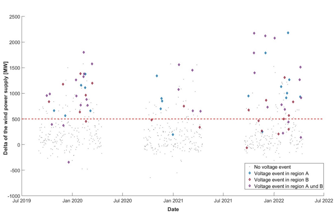
Figure 6 - Delta of the wind power supply between 6:00 a.m. and 6:15 a.m. in Germany
for the winter months (September - April)
Further cause-effect relationships in the data could be identified from similar analyses, so that key input parameters that are frequently associated with the occurrence of voltage events could be derived:
- High offshore and onshore wind power feed-in
- Low total power feed-in of conventional power plants in regions A and B
- High grid load
- High power transfer from the north to the south of Germany, resulting in a high reactive power demand of the lines
- High reactive power provision of conventional power plants (over-excited operation to increase voltage)
The identified correlations reflect a grid state, in which there is a sudden high reactive power demand due to a high delta in wind power feed-in, a high grid load and a high resulting power transfer, which can only be covered by few voltage supporting power plants. This grid state is often particularly pronounced at 6 a.m.
3. Selection of a forecast method for voltage drops
A practical forecast method that predicts voltage drops is needed to warn operators of situations that might jeopardize grid security in advance. Such a practical forecast method is required to make clearly understandable and reliable statements regarding voltage drops based on available forecast data with adequate advance notice. Therefore, in Chapter 3.1 the availability of existing input data is described and an execution time for the forecast is derived. Chapter 3.2 presents various potential forecast methods and the challenges that exist when forecasting voltage drops. In Chapter 3.3, the methods presented are compared with each other regarding forecast quality as well as practicality. The functionality of the forecast method which was identified as the most suitable for the integration in an operational process based on this comparison is described in Chapter 3.4.
3.1. Availability of input data and execution time
In contrast to the analyses presented in Chapter 2, only ex-ante available information can be used for the forecast. Thus, the forecast model depends on inputs, which are themselves forecasts of various fundamental data. The time at which the forecast is executed determines the predictors that can be used and influences the expected forecast quality. In general, the greater the time interval between forecast and real time, the smaller the number of available predictors and the higher their forecast uncertainty. Nevertheless, there must still be enough time after the forecast has been generated to be able to react to the result, e.g. start-up of power plants for voltage support. Taking these constraints into account, the most suitable execution time is set at 4:30 p.m. of the previous day (day-ahead). The predictors available in this time range and their resolution are listed below, taking into account all of the influencing factors deemed relevant in Chapter 2.3:
- Control area demand and vertical load of each German TSO (day-ahead, for each hour of the next day)
- Wind power infeed and PV power infeed of each German TSO (day-ahead, for each hour of the next day)
- Temperature for different regions (day-ahead, for each hour of the next day)
- Economic dispatch for each power plant according to power plant operators schedules (day-ahead, for each quarter hour of the next day)
- Day-ahead spot market prices (day-ahead, for each hour of the next day)
3.2. Potential forecast methods and forecast challenges
An important requirement for operational forecast tools is that they provide clearly understandable warnings, which is why the chosen forecast method should make yes/no-statements regarding the occurrence of voltage events. Therefore, different binary classification methods, which are supervised machine learning methods that categorize data into one of two classes, were analysed for the selection of a potential forecast method. In contrast to forecasting continuous values (e.g. solar power feed-in, temperature, etc.), only binary statements are made.
Three of the most widely used supervised classification methods were taken into consideration for the problem of forecasting voltage drops:
- Support Vector Machine (linear und gaussian) [5]
- Random Forest [6]
- Logistic Regression [7]
All methods were evaluated using an implementation from the Matlab Statistics and Machine Learning Toolbox [8].
The biggest challenge in predicting voltage drops is the very small number of only 262 voltage events. In the case of a forecast model with hourly resolution, this would result in 262 hours with event are compared to 22,730 hours without event. A forecast model which always predicts no voltage event for every application would thus have a high forecast quality of 98.9%. Typically, when training classification methods, a training data set is provided to the individual models, on the basis of which the respective methods are parametrized. The training data set should consist of equal parts of points in time with and without voltage events. To achieve this, a so-called "class balancing" is necessary. There are several methods to perform class balancing. Typical methods are oversampling (copying samples of the class with a lower proportion) and undersampling (deleting samples of the class overrepresented). In this work, a hybrid of these methods is used. Depending on the temporal resolution chosen, between 91,968 15-minute values and 958 days are available for training. However, using 15-minute values leads to a very unbalanced training data set. In this case, the high degree of balancing results in a high dependency of the training data on the stochastic balancing outcome. Therefore, the temporal resolution of the forecast is reduced to days. For the forecast on a daily basis, daily mean values and daily maximum and minimum values are determined for the predictors.
Another challenge is the need for separation between training and test data, as this further shrinks the available training events. A separation between training and test data is fundamentally required in the field of machine learning in order to verify the ability of the models to generalize. In this case, the models are first parameterized using a training data set. However, the prediction quality is not evaluated on the basis of this training data, but on the basis of the test data. This is to avoid that the training data are simply reproduced ("learned by heart") and the so-called "overfitting" occurs. Again, there are different approaches to separate training and test data. In the context of this work the procedure of k-fold-cross-validation is used, in which a part (e.g. 20 %) of the total data is used as test data and the procedure is repeated under exchange of the test data (with 20 % 5 times). The default value is k = 10 [9]. In addition, a voltage drop forecast is only of practical relevance if the region of occurrence can also be determined. For this purpose, two forecast models must be created instead of one, since two main regions (A and B) for the occurrence of the voltage drops could be identified in the spatial analyses according to Chapter 2.2. This further reduces the available training events, since some voltage drops only occur in one region at a time. As a final challenge, the models have a high number of possible predictors available in addition to the small number of training events. This combination of few training events and many predictors further increases the risk of overfitting. In addition to overfitting, the prediction quality can also be lowered by the use of collinear predictors. To counter this, the number of predictors used is kept to a minimum.
3.3. Comparison of forecast methods
The selection of the most suitable forecasting method is based on the aspects of practicality and forecasting quality. The number of predictors is used to estimate the practicality. Since the procurement of data from many different predictors from different data sources is very time-consuming and involves a high risk of failure, the number of predictors should be kept as small as possible. In addition, as described in Chapter 3.2, this reduces the risk of overfitting and collinearity of the predictors.
When reducing the number of predictors, care must be taken that the forecasting model used is not too simple in order to reflect the complexity of the underlying principles.
For this purpose, the number of predictors used is successively reduced and the forecast quality is observed. In order to determine the order of the predictors to be removed, the relevance of the individual predictors for the quality of the forecast result is rated. The method used for this is described in more detail in Chapter 5.2. and illustrated in Figure 13.
The evaluation of the different forecast methods is carried out independently for both regions A and B. As an example, only the results for Region A are shown in Figure 7, where validation accuracy is defined as the number of correctly predicted voltage events divided by the total number of predictions.
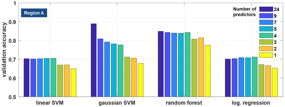
Figure 7 - Forecast quality as a function of the number of predictors
The linear SVM and logistic regression methods show a slight improvement in the quality of forecasts up to a reduction to four predictors. The random forest method shows an almost constant forecast quality up to a reduction to four predictors. With fewer predictors the quality decreases significantly but the overall forecast quality is at a significantly higher level. The gaussian SVM method shows a steadily decreasing forecast quality. This indicates that the gaussian SVM method, unlike the others, tends to be affected by overfitting. The improvement of the other methods with fewer predictors is probably due to the reduced collinearity of the predictors.
Based on this analysis, the random forest method was chosen for region A. The forecast quality of the selected forecasting method was then evaluated using a confusion matrix. A detailed description of the evaluation procedure is provided in Chapter 5.3.
Since the results for region B were very similar, the random forest method was chosen for region B as well. The operation of the selected forecasting method is briefly described in the following chapter.
3.4. Functionality of the chosen random forest method
The random forest method starts from so-called decision trees. With the help of these trees, classifications of the input data can be carried out by simple yes/no queries. Depending on the input data, a certain path within the tree is traversed, at the end of which the decision between event or no event is made. How such a classification of the input data can look like is exemplarily shown in the left part of Figure 8.
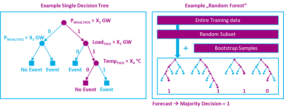
Figure 8 - Schematic structure of decision trees (left) and the random forest method (right)
Very efficient algorithms exist for the generation or "growth" of decision trees, which can be used to determine the optimal sequence of queries to match a known result. Since this method tends to overfit, it is rarely used in practice. To prevent this effect, the random forest method generates a large number of parallel decision trees (hence "forest"). During growth, only a randomly selected subset of the training data is available to the respective trees (hence "random"). Thus, each tree grows in an individual way and the ability of the method to generalize is strengthened. Furthermore, the method is supplemented by randomly generated variations, so-called bootstrap samples. This guarantees that the procedure reacts robust in the later prediction phase even in case of slight deviations of the input data. After completion of the learning phase described above, the method can be used for forecasting. The input values pass through the respective queries in all trees and each tree arrives at a binary decision (event/no event). The majority decision across all individual trees defines the overall forecast result [6].
4. Application of the forecast method in an operational process
An operational process called uDrop was implemented in 2019 to warn operators of voltage drops day-ahead using the selected forecast method described in Chapter 3.4. In this context, a forecast with hourly resolution was developed in addition to the daily forecast. The development of the hourly forecast is briefly described in Chapter 4.1. Chapter 4.2 gives an overview of the workflow of the operational process uDrop. In Chapter 4.3, countermeasures that can be planned by the operators based on the results of the process are presented.
4.1. Development of an hourly forecast
In order to facilitate the coordinated use of countermeasures to prevent voltage collapses for operators, an hourly forecast method was developed in addition to the daily forecast method described in Chapter 3.4. As with the daily forecast, the greatest challenge in developing an hourly forecast method is the low number of training events. Based on the identification method described in Chapter 5.1, the hourly voltage events that occurred from 2018 to 2022 were identified. In this evaluation, 262 voltage events that took place at the change of the hours could be detected. In contrast, there are 22,730 hours without a voltage event, leading to a ratio that makes the hourly prediction even more difficult than the daily prediction.
For this reason, a set of 100 random forest forecast models is trained for every hour of the day for both regions A and B, each of which making its own binary decision regarding the occurrence of a voltage event (yes/no-statement). Thereby, the hourly forecast delivers a value between 0 and 100 for each hour of the following day, which can be interpreted as the probability of occurrence of a voltage event for that respective hour. Hourly values above 50 are considered to have an increased probability of voltage events.
Figure 9 shows the results of an exemplary execution of the daily forecast for Region A. Considering this example, the highest probability for a voltage event can be seen at 6 am. As the probability for voltage events is higher than the threshold value of 50 % for the hour changes at 07:00, 10:00, 17:00 and 18:00 as well, in this example operators should also be cautious regarding these timesteps.
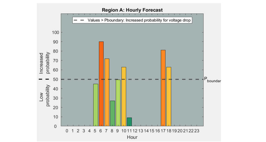
Figure 9 - Exemplary presentation of the results of the hourly forecast for Region A
4.2. Workflow of the operational process
The flowchart of the process uDrop is shown in Figure 10.
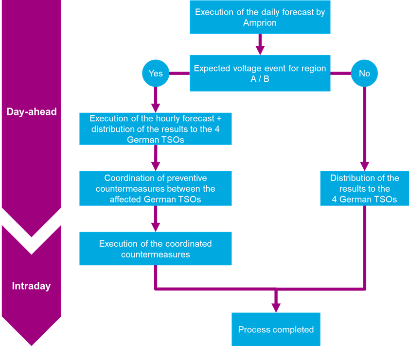
Figure 10 - Flowchart of the uDrop process
The first process step is the execution of the daily forecast at 4:30 p.m. day-ahead for the following business day by the operators of Amprion’s Operational Planning (OPL). As a result, the forecast makes a yes/no statement about whether or not a voltage event is expected on the following day for both regions A and B. If no voltage event is predicted for either region, the other German Transmission System operators are informed about this and no countermeasures to prevent voltage drops must be planned day-ahead. If a voltage drop is expected for at least one of the regions, the hourly forecast is carried out by the operators of Amprion GmbH to determine at which hours of the following day voltage drops are most likely to occur. Based on these results with a high temporal solution, the operators of the affected German Transmission System Operators can plan countermeasures against voltage events in a coordinated manner. The results of the forecast are provided to the operators via an application which is shown in Figure 11. Next to the forecast results, the application offers the possibility to show the input data in high temporal resolution such as wind power feed-in or the dispatch of conventional power plants. This enables operators to understand the causes of the voltage events easily and take them into account when planning countermeasures. In the next chapter, the countermeasures available to operators to prevent or mitigate the voltage drops are summarized.
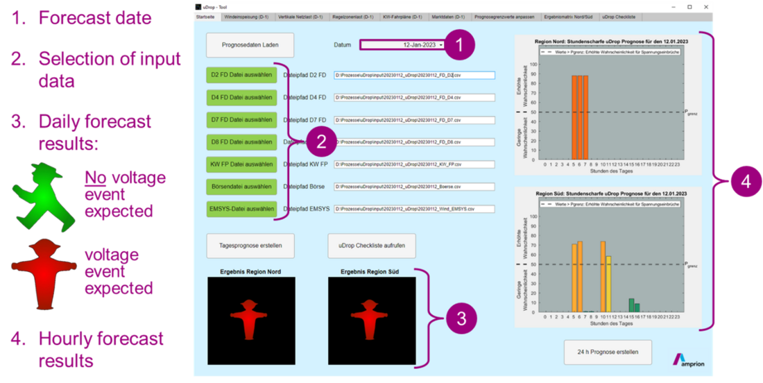
Figure 11 - Matlab application for executing the uDrop forecast and visualizing the results
4.3. Countermeasures to prevent voltage drops
In principle, all countermeasures permissible under the regulations for avoiding operating voltage range violations can be carried out by operators both in operational planning and in real-time operation. The available countermeasures and the order in which they are applied are described in the common handbook available at each TSO [10]. The available countermeasures are divided into three categories:
- Grid related measures
- Market related measures
- Emergency measures
Grid related countermeasures include the use of reactive power compensation systems such as MSCDNs and reactors, the adjustment of the reactive power supply of power plants, synchronous condensers or STATCOMs and should be applied first. Moreover, market related measures such as redispatch or the use of special power plants constructed for grid safety can be carried out for voltage support. In emergency cases, it is also allowed to block automated regulation of coupling transformers and to disconnect loads or generators in the context of emergency measures.
The operational use of these measures is always evaluated depending on the grid situation. The decision on the use of individual measures is left to the operators, considering proportionality and effectiveness. Based on previous experience, the use of cost-intensive redispatch solely based of an expected voltage drop has not been necessary so far. Instead of this, grid related measures are carried out in order to keep the voltage robustness of the grid as high as possible and to damp voltage drops as far as possible. This is achieved in operation by avoiding topological grid weakening (no disconnection of lines, transformers and couplings) and the use of voltage-supporting units (converters, STATCOMs, synchronous condensers). In addition, a high operational voltage level is approached for the hours identified as critical, e.g., by preventively switching on capacitors and switching off reactors. Exceptions to this are MSCDNs and reactors with automatic switching.
5. Monitoring and further developments of the forecast process
Since uDrop is an operational process that is used as decision support by the operators of the German Transmission System Operators, it is necessary to continuously monitor and further develop the process and the forecasting quality. The procedure for monitoring and further developing the process is carried out at least once a year and is shown in Figure 12. To determine the forecast quality, it is necessary to identify the voltage events that occurred in the past and to compare them with the forecast results. The identification procedure developed for this purpose is described in Chapter 5.1. In a next step, the causes for undetected or incorrectly predicted voltage events are analysed . Based on these analyses, model improvements to increase forecast quality are carried out, e.g. adjustments regarding the selection or number of used predictors. Model improvement and fine-tuning are especially important for this process as the used forecast model is a supervised machine learning algorithm, which makes predictions based on training data and not on fundamental relationships. As the characteristics of the Transmission System are changing over time, e.g. by construction and destruction of power plants, lines and transformers, change of topology or changed behavior of market participants, training data must be adapted accordingly. Model improvement and fine-tuning of the process are described in Chapter 5.2. With supervised machine learning algorithms, trained models must be evaluated against test data to ensure robustness. This evaluation is especially important for an operational process and is therefore carried out before each operational implementation by Amprion GmbH. Chapter 5.3 exemplary describes such an evaluation for the year 2022.
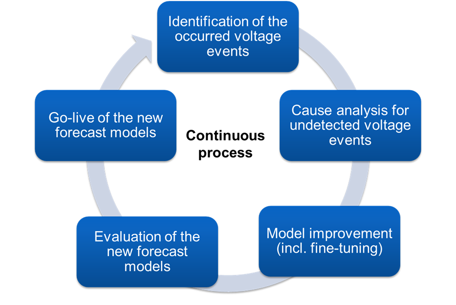
Figure 12 - Continuous process for the further development of the forecasting models
5.1. Identification of voltage events
The continuous determination of voltage events is necessary to determine and improve forecast quality. The biggest challenge in this process is the differentiation between fast voltage changes that are caused by active power flow changes and those that are caused by grid related measures. The identification procedure developed for this purpose consists of 3 steps and is described in more detail below:
- Determination of all voltage drops higher than 7.8 kV within 10 minutes & filtering of measurement errors and change of busbars.
- Determination of the effect of grid related measures on voltage magnitude for identified voltage drops.
- Determination of voltage events as hypothetical voltage drops without realised grid related measures.
Firstly, all voltage drops that exceed the threshold value of 7.8 kV withing 10 minutes are calculated based on measured values which are available in a temporal resolution of 3 seconds. In the process, outliers that occur due to measurement errors or the change of busbars are filtered out algorithmically and not considered further.
In the next step, the effect of grid related measures for voltage support that were carried out at the times of the identified voltage drops is determined. For this purpose, historical data models that reflect the grid state at the time of identified voltage drops and cover the observability area of Amprion GmbH are considered. For these data models, power flow calculations are performed to determine the voltages occurred at the busbars in reality. Subsequently, these data models are modified so that grid related actions are extracted from the data models and power flow calculations are carried out for the modified data models as well. The voltage magnitudes obtained with modified power flow calculations can be used as an indicator of how the voltage drops would have occurred without grid related measures, but only due to active power flow changes.
In a last step, differences between voltage magnitudes that occurred in reality and voltage magnitudes obtained with modified data models are calculated. Those values are added to the voltage drops that were identified in the first step, so that hypothetical voltage drops without realised grid related measures are obtained. In this way, some of the absolute values of the initially calculated voltage drops are reduced, so that it can be concluded that these voltage drops were caused by grid related measures. On the other hand, some absolute values of voltages drops are increased as the effect of voltage increasing countermeasures is extracted. All voltage drops that exceed the value of 7.8 kV after the execution of this last step are considered as voltage events, which are voltage drops that exceed the threshold value of 7.8 kV withing 10 minutes and are caused by fast active power flow changes.
Applying this identification method, a total of 262 voltage events could be identified in the period from 2017 to 2022 as already mentioned in Chapter 2.1.
5.2. Continuous Root cause analysis and model improvement
The root cause analysis described in Chapter 2.3 has been conducted continuously since the initial forecast model went into operation in 2019. In the process, it is regularly questioned whether voltage events were not detected or incorrectly predicted due to the parameterization of the forecast models or the weighting and selection of the predictors. For example, in addition to daily mean values, daily maxima and minima are also considered as predictors in the forecast models to be able to consider wind peaks or times in the daily course with particularly low power plant infeed. The weighting of these predictors varies and depends on the influence on the forecast quality. In the forecast models from winter 21/22, the mean-based predictors were more heavily weighted than the maxima- or minima-based predictors, which meant that some events could not be detected. Based on this finding, more focus was placed on the maxima- and minima-based predictors when weighting the predictors for winter 22/23.
In order to be able to estimate the optimal weighting and selection of predictors, the random forest procedure provides a rating of the relevance of the individual predictors for the quality of the forecast result as a partial result [8]. An exemplary estimation of the predictor importance for Region A is shown in Figure 13. The 4-7 predictors with the highest influence on the forecast quality are used to generate the forecast. In this range, the forecast results are generally stable. With more than 7 predictors, the risk of overfitting increases. With 3 or fewer predictors, the model used is too simple to reflect the complexity of the underlying principles (cf. Chapter 3.3).
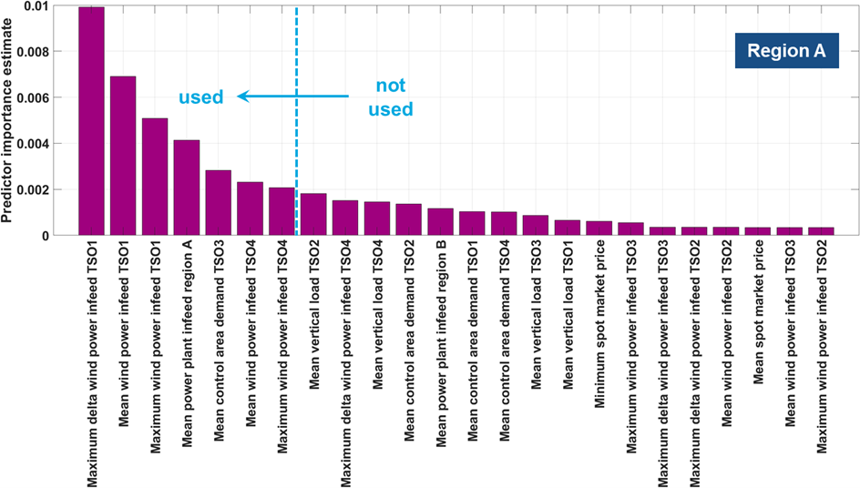
Figure 13 - Predictor importance estimation of the random forest procedure
Furthermore, there are also voltage events that were not detected or incorrectly predicted, regardless of the weighting and selection of the predictors. The reason for this is that the cause-effect relationship behind the voltage events has not yet been clearly explained and not all influencing variables that lead to the occurrence of the voltage events are known. An important part of the continuous cause analysis is therefore the search for new influencing variables or predictors.
In addition to the search for new predictors and the estimation of the weighting and selection of the predictors, there are various other fine-tuning options when using the random forest method. One possibility for fine-tuning is to limit the available degrees of freedom of the individual decision trees by specifying the maximum number of permissible splits. This can reduce the risk of overfitting.
Another possibility for fine-tuning is the use of a cost matrix, which can be applied to the forecast model during training. This makes it possible to control the sensitivity of the forecast in a targeted manner to give greater weight to undetected events than to event warnings to ensure safe grid operation [8]. A possible cost matrix that can be used in the context of fine-tuning is shown in Table I.
| Voltage event predicted | Voltage event not predicted |
|---|---|---|
Voltage event occurred | 1 | 2 |
Voltage event not occurred | 1 | 1 |
In this cost matrix, an undetected event is weighted twice as heavily as a wrongly predicted voltage event.
5.3. Evaluation and commissioning of a new forecast method
For the evaluation of the forecast models, data from the winters 17/18 - 20/21 were used for training. The data from winter 21/22 were used as a test data set. The number of predictors was limited to 5, as the best forecast quality could be achieved in the model improvement phase for this parameterization.
Applying the final models to the test data of winter 21/22, the forecast quality shown in Figure 14 was achieved for Region A. The results for region B correspond to those of region A and are therefore not explicitly listed in the following.
To estimate the quality of the forecast, the following two questions are particularly relevant:
- For how many occurred events a warning was given?
(Number of predicted and occured events / number of all occured events).
- In how many cases was an event warning followed by an occured event?
(Number of predicted and occured events / number of all predicted events)
The results are presented in the form of a "confusion matrix". The interpretation of the confusion matrix is described in detail in the figure.
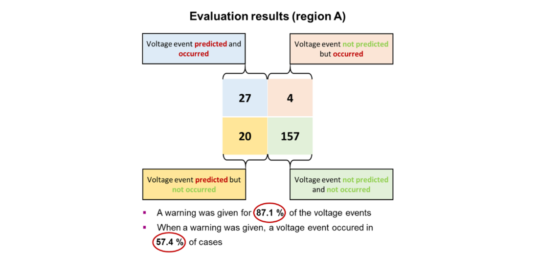
Figure 14 - Confusion matrix of evaluation results for region A
The model for region A acts more risk averse and has a tendency to give warnings even though there is no voltage event. However, this is in accordance with the objective of safe grid operation.
Since the uDrop forecast went into operation in September 2019, the forecast models have been regularly improved with the aim of continuously increasing the forecast quality. The current forecast quality of the forecast models from winter 22/23 is illustrated in Figure 15. For comparison, the figure also shows the forecast quality of the initially created forecast model from winter 19/20.
As the figure shows, the developments of the last few years have led to a significant reduction of false predicted events, while at the same time the detection rate of the events has remained almost constant. When a warning was given in winter 22/23, a voltage event occurred in 66.7 % of cases. In winter 19/20, it was only in 38 % of the cases. Two main drivers can be named for the improvement in forecast quality. The first main driver for improvement is the consideration of the hourly delta of wind power generation as a new predictor of the forecasts, which was added in 2021 (cf. Chapter 2.3 figure 6). As a second main driver, the increasing training data set over time has contributed significantly to the improvement of forecast quality.
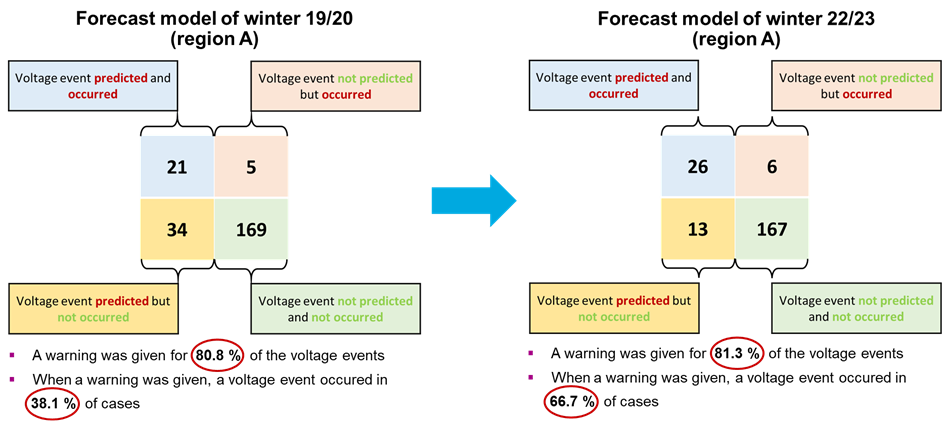
Figure 15 - Comparison of forecast quality from winter 19/20 vs. 22/23 for region A
Overall, the development of the forecast quality shows that the regular monitoring and further development of the uDrop process leads to improved results. The described model is able to predict voltage events with a very high probability. This means that first reliable voltage forecasts can already be carried out on the day-ahead.
6. Conclusion
Within the scope of this work, short-term voltage drops in two different regions (A and B) in the German transmission grid were analysed in detail. The causes for the occurrence of these voltage events were investigated by statistical analyses.
Based on the results of the analyses, two separate forecast models were developed, which allow an independent daily forecast of the voltage events in both regions. In order to facilitate the coordination of countermeasures, the daily forecast was additionally extended by an hourly forecast. The forecasts are carried out with input data that are already available day-ahead, so that there is enough time to prepare for potential voltage events in both regions.
Since 2019, the forecasts have been part of the operational processes of the four German Transmission System Operators. One of the biggest challenges for the quality of the forecast is the constant change in the Transmission System, e.g. due to the expansion of renewable energies and the reduction of conventional power plant capacity. To address this challenge, the forecast quality is being continuously monitored and the forecast models are at least annually improved.
Acknowledgement
The voltage drop prediction presented in this paper was originally developed in the year 2019 in a study [4] conducted by ef.Ruhr GmbH and commonly funded by the TSOs 50Hertz Transmission GmbH, TenneT TSO GmbH, TransnetBW GmbH and Amprion GmbH. Since then, further analyses, developments and tuning of the method were carried out by Amprion with support from the other German TSOs, particularly concerning data delivery.
References
- 50Hertz Transmission GmbH, Amprion GmbH, TenneT TSO GmbH, TransnetBW GmbH, "Notwendigkeit der Entwicklung Netzbildender STATCOM-Anlagen," pp. 2-3, December 2020, [Online].
- The Federal Goverment, "Technical Instructions on Noise Abatement," 2017, [Online].
- 50Hertz Transmission GmbH, Amprion GmbH, TenneT TSO GmbH, TransnetBW GmbH, "Deutsches Grenzwertkonzept," pp. 18-20, November 2021, [Online].
- S. Kippelt, "Analyse und Prognose von Spannungseinbrüchen im deutschen Übertragungsnetz," pp. 4-29 (non public), Dortmund, Germany, October 2019.
- N. Christianini, J. Shawe-Taylor, “An Introduction to Support Vector Machines and Other Kernel-Based Learning Methods,” Cambridge, UK, Cambridge University Press, 2000.
- L. Breiman, "Random Forests," pp. 5-32, October 2001.
- D. Hosmer, S. Lemeshow, "Applied logistic regression," vol. 2, New York: Wiley, 2000
- The MathWorks Inc., "Matlab Statistics and Machine Learning Toolbox Version 12.0," 2023, [Online].
- T. Hastie, R. Tibshirani, J. Friedman, "The Elements of Statistical Learning," vol. 2, New York: Springer, August 2008, pp. 241-245.
- 50Hertz Transmission GmbH, Amprion GmbH, TenneT TSO GmbH, TransnetBW GmbH, "Handlungsleitfaden der dt. ÜNB zur Anwendung der Maßnahmen nach §13 Energiewirtschaftsgesetz," pp. 18-24, July 2023.