Blackstart of 100% IBR Dominated Power Systems: Ensuring Small-Signal Stability in each Stage
Authors
Stavros KONSTANTINOPOULOS, Deepak RAMASUBRAMANIAN, Vikas SINGHVI
Electric Power Research Institute (EPRI), Knoxville, Tennessee, USA

Summary
During power system blackstart (BS), the topology of the energized system changes drastically with each grid element coming online. These changes, along with changes in loading and generation mix, can alter the dynamics of the islanded “live” system. Currently, the dynamic stability of power systems in such early stages of the restoration, is assessed mainly by extensive EMT simulations. EMT simulations can offer great insights on the time-domain response, but offer little information on the root cause of instabilities, when those arise. In systems dominated by Inverter-Based Resources (IBRs), interactions with the network and higher frequency dynamic instabilities can also arise. In this work, we examine how the dominant dynamics of the system change during a sample early restoration process, and how an eigenvalue-based stability analysis can offer insights into the dynamics of energized network in each step. In addition, via participation factor analysis we identify the responsible control loops and equipment. For each examined restoration stage, we demonstrate that via parameter sweeps, safe parameterizations can be established for the entirety of the process. In addition, we describe how we construct power system dq models in a modular fashion, in order to interface individual components and construct the full closed-loop system.
1. Introduction
Small-signal stability of power systems has been a wellstudied topic in the past decades. The control and equipment interactions, as pertaining to their impact on rotor angle interarea stability, were well understood and a plethora of methods to analyze them has been proposed and used in practice. In most cases, utilization of positive sequence RMS models, omitting network dynamics, was sufficient to capture such behavior and subsequently be utilized for analysis, control synthesis or tuning. As power systems are transitioning to the era of IBR generation, traditional RMS small-signal analysis approaches have proven insufficient to capture all the dynamics of interest [1]. This can be attributed to the higher frequency dynamics exhibited by VSC-based generators, affecting bandwidths simply not modeled in most positive sequence environments. In addition, as power systems will begin introducing grid-forming (GFM) IBRs, traditional rotor angle dynamics might begin to shift, as the effective inertia will no longer be tied to the physical masses behind the conventional generator, but will be subject to tuning, in order to meet specified stability criteria. Extensive work has been carried out to analyze the small-signal stability of systems with GFM and grid following (GFL) IBRs [1], [2], [3], [4]. For the purposes of analyzing the stability of IBR dominated systems, two major approaches have been utilized in literature. The first is the traditional state-space methods [1], [2], [5] and the second, stability criteria based on impedance-based analysis [6], [7], [8]. Smallsignal analysis in the power system blackstart scenario has not received much attention. Authors in [9] include a smallsignal stability margin, along other indices, to asses the overall stability of the system across all stages of the blackstart process. In [10], the authors introduce a reduced order model of a decentralized microgrid to asses its dynamic stability during blackstart. Authors in [11], give an in-depth review of all the challenges and methods used to analyze the small-signal stability of large power systems, with emphasis on modular construction of such models.
Establishing a blackstart process is an already involved process, that requires extensive simulations across all stages, to ensure feasibility, in addition to adequate system performance [12], [13], [14]. However, the dynamics of IBR dominated systems in such scenarios have not been sufficiently studied nor are well understood. Blackstart in itself has two main challenges from a dynamics perspective. The first is that the grid presents much sparser structure. Secondly, in each stage, as more lines, loads and generators are brought online and the topology and load/ generation mix changes, significant shifts in dynamics can occur. Without sufficient methods to analyze the small-signal properties of a system during blackstart in the EMT scale, identification of underlying causes, mitigation or retuning can be challenging. In addition, given the computational burden of EMT simulation, simulating the blackstart process for each examined dynamic instability remedy or retuning, can be a time consuming task. In this work, we provide a framework of how eigenvalue-based analysis can be a valuable tool to scan for stability of IBR parameterizations across all stages of blackstart, in order to establish a “safe” parameter set. If no such parameter set can be found, the operator can use all the established tools of linear system analysis, like participation factors, to identify responsible controls or equipment, retune them, and establish a gain schedule for each step of blackstart. We also outline how a small-signal model of the system can be built in a modular fashion, without any simplifications.
2. Power system DQ modeling
In this section, the dynamics of each individual component are described. For the purposes of this study, the models are assumed as white-box, with total visibility of controls. However, in situations where the models are “black-box”, i.e., there is not visibility of controls, the methodology can be slightly altered. In [15], the readers can find an approach on how to integrate identified linear models of black-box IBR models, into a larger small-signal analysis framework.
2.1. Photovoltaic Plant Model
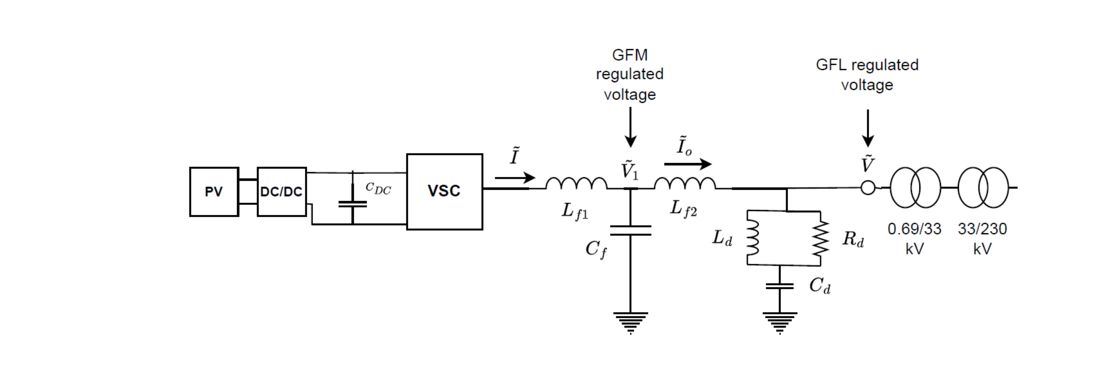
Figure 1: PV Plant Topology - Similar to [16]
For the purposes of this study, the IBR plants are assumed to be photovoltaic (PV) based. Since the plants examined are in the scale of 100s of MW, they should be expected to be comprised of multiple individual inverters, coordinated by plant level controls. However, for system level studies, aggregate models are commonly utilized and are adequate to demonstrate our methodology geared towards screening smallsignal stability during blackstart. Of course, other type of IBR plants can be considered and included in our formulation. In this study, the PV plants are assumed to be operated in DC voltage control mode. This implies that a boost converter regulates the DC capacitor voltage to a set-point by controlling its duty cycle and delivers the required power from the PV cell array. The boost converter is assumed in its averaged representation:
(1)
For the purposes of linearization, the PV array is represented by a VI curve and during linearization the sensitivity of voltage to current around the operating point is utilized. The model incorporates a DC side capacitor and the 2 level VSC is represented by an averaged model. The dynamics of the DC side capacitor can be summarized as
(2)
According to the averaged representation, the voltages of the VSC are derived as
(3)
where mi is the i − th phase modulation signal as generated by the VSC’s controls. The voltages are cast in the dq frame of reference. On the AC side of the VSC, there exist an LCL filter and at the terminals a shunt filter. The AC and DC sides are interfaced via instantaneous power conservation [17] i.e.,
(4)
(5)
2.2. Frame of Reference
All quantities in the following control structures are assumed in the IBR’s local frame of reference (FOR). Any quantity defined in the system’s synchronous frame of reference will be rotated by an angle − θ, dictated by the IBR’s synchronization loop (droop or PLL) as
(6)
where quantities with a ˜ are defined in the system’s FOR.
3. Grid-forming Converter Controls
The GFM controls utilized in this work, incorporate the low-pass filtered droop paradigm [2]. The controls of the VSC are set to control the LCL filter capacitor voltage. The voltage control is achieved via a multi-loop control with the outer voltage control loop dictating the current references and the inner loop regulating the filter current [18]. The synchronization loop is realized as
(7)
where θ is VSC the internal angle, realized at the LCL filter capacitor, TP is the time constant of the power filter, KP is the active power droop gain, P∗ is the active power set-point and P is the VSC active power output. In addition, a QV droop is incorporated to allow reactive power sharing. The d-axis reference is dictated by
(8)
where V0 is the voltage reference, KQ is the reactive power droop gain, TQ is the reactive power droop time constant and Q is the reactive power output. The q-axis reference is set to 0. s is the Laplace complex operator. The voltage controls are realized as
(9)
(10)
where are the dq current references, Kpv, Kiv are voltage control proportional and integral (PI) gains, respectively. Vd, q are the dq voltages of the capacitor of the LCL filter. F is the current feed-forward (FF) gain and Cf is the LCL filter shunt capacitance. ωs is the synchronous speed in r/s. Finally, the VSC modulation signals, in the dq frame of reference, are generated by the current controller, defined as:
(11)
(12)
where Lf1 is the inductance of the first segment of the LCL filter. It should be noted that all currents and voltages are low-pass filtered by a first-order filter, before used in any control loop. However, the currents/ voltages are not filtered before used for P and Q calculations as the powers are filtered separately.
3.1. Grid-following Converter Controls
The GFL controls utilized in this work, adopt the plant and inverter, two-level control structure. The plant controller is set to regulate the terminal voltage of the IBR (or can be compensated to regulate a point further in the network). The plant level voltage controller synthesizes a reactive power command as
(13)
The command is then low pass filtered to emulate the delays in communication and other filtering. A Pad´e approximation formulation of the plant control delay will be examined in a subsequent section [19]. Due to the delay of the plant controller and other signal filtering, the overall response should be expected to be slower than the IBR level controls which in turn realize the reactive power reference.
(14)
the d, q axis current references are then generated, at the inverter level, as
(15)
(16)
The current controls are then realized in the same manner as the GFM controls. Finally, the synchronization with the grid is achieved via a PLL, realized as
(17)
where notation implies the estimated terminal bus voltage angle.
3.2. Transmission Line Modeling
For the purposes of modeling the transmission lines of the system, a distributed T-section model as described in [20] is utilized. Unless specified, two T-sections are usually utilized. Due to space limitations, the reader can refer to the reference for the full description of the model.
3.3. Transformer Modeling
In our work, transformers are modeled as inductors, neglecting the shunt core inductance, losses and saturation. Saturation can play a significant role in large signal disturbances, but for our investigation, the transformer is assumed to operate far from the saturation point. Another phenomenon that is particularly relevant to blackstart studies, are inrush currents during transformer energization. Such phenomena fall under the large-signal umbrella and hence should be evaluated by tools suitable for such analysis.
3.4. Induction Motor Modeling
Induction motors (IM) are modeled by a 5th order model following the formulation of [17]. This model incorporates four flux states for the dq axis of both the stator and rotor and a mechanical state for the rotor speed. In addition, shunt capacitors are assumed at the motor plant, in order to correct the power factor to 0.95 lagging. The mechanical load is assumed to be of the quadratic speed to torque form
(18)
3.5. Passive Loads
Passive loads are modeled by shunt parallel RL components. The dynamics of an RL load can be summarized as
(19)
(20)
where RL, LL are the load’s resistance and inductance and Id,q are the terminal dq currents assumed to flow into the load. The voltages across the inductor can be simply calculated by calculating the voltage across the resistor since the input current is assumed as the independent variable. This model will be used to emulate the constant impedance part of the load. In our case study, it will be used in conjunction with motor loads (not on the same bus), to yield a more realistic load mix.
4. Modular Network Construction
Each component is linearized around its operating point, taken from a power flow solution. Network elements will be two port state-space objects while loads and generators will be single port objects (1 port implies a pair of dq quantities). Network elements are represented in admittance form (voltage is the input and current the output) while passive loads, motors and generators are represented in impedance form (current as input and voltage as output). Loads and generators are always assumed to be interfaced with the network via a transformer. The network is constructed according to Algorithm 1.
5. Analysis Methodology
The analysis of the next section will be based on state-space analysis methods. Poles will be evaluated for their stability across various parameter sets, in addition to their damping ratios. Furthermore, participation factors of each mode will be calculated [21], in order to identify participating states in each mode. For each mode, states will be deemed as participating if their corresponding participation factor in the mode, is at least 10% of the magnitude of the maximum participation factor of the mode.The system modes that will be considered are below 500 r/s (unless specified otherwise), as there will always exists high frequency/ low-damping modes, that are
| Algorithm 1 Network Construction Algorithm | |
|---|---|
| 1: | procedure NETWORK CONSTRUCTION |
| 2: | for each bus in network do |
| 3: | Identify elements connected to bus |
| 4: | Close loop of appropriate ports via circuit equations |
| 5: | Create combined (A,B,C,D) matrices for new hyper-component |
| 6: | end for |
| 7: | Output N et state-space object |
| 8: | end procedure |
| 9: | procedure GENERATOR-LOAD STATE-SPACE OBJECT CONSTRUCTION |
| 10: | for each port of N et object do |
| 11: | Append load or generator model connecting to the port, to Gen object |
| 12: | end for |
| 13: | end procedure |
| 14: | Close loop via feedback of N et via Gen |
not really observable in most cases in the step response. These modes will be reported in subsequent sections if they appear to be unstable or if notable changes in damping occur during parameter sweeps.
Finally, the results will be depicted in a parameter sweep format. In particular, for two varying parameters, the stability will be assessed by the location of the closed-loop poles, classified as well-damped (deemed as stable in the heatmaps), under-damped (less than 5% damping coefficient) and unstable. The condition will be color-coded and plotted on an interpolated heat-map, so the reader can get a clearer picture of which parameter sets fall under which category. The parameter grids examined will be 15 × 15. The stability regions will be presented by interpolated heatmaps, as a visual aid for ease of interpretation of the results. Due to the finite numbers of points considered in each sweep, the boundaries of those regions might present as ‘step-like’ transition. For verification of results, sample time-domain EMT simulations will be presented to verify the results of our small-signal analysis, for a few of the examined blackstart stages.
The analysis of the test system for each stage of the blackstart process, assumes a predicted load and generation, which is the operating point around which the small-signal analysis is carried out. For each stage, additional loading and generation allocations can be examined in order to assess the robustness of the system’s small-signal stability properties.
6. Blackstart process
In this section we will describe each stage of a sample blackstart process. In each stage, the topology changes, generation mix and loading will be described, in addition to the parameterization of the new elements.
6.1. Blackstart Procedure Small-signal Stability Screening
During the blackstart operation, an energization plan must be established. During each stage, the elements and their respective parameters must be known in order for the models to be constructed. In addition, the estimated loads to be connected and their compositions must be provided. Then the procedure can be carried out as described in Algorithm 2.
| Algorithm 2 Blackstart Small-Signal Screening | |
|---|---|
| 1: | procedure BLACKSTART SMALL-SIGNAL SCREENING |
| 2: | for each stage do |
| 3: | Read model parameters |
| 4: | Solve power flow |
| 5: | Construct small-signal model |
| 6: | Screen for small-signal stability |
| 7: | if System Unstable or Poorly Damped then |
| 8: | Identify responsible loop via participation factor analysis |
| 9: | end if |
| 10: | end for |
| 11: | end procedure |
6.2. Test System
For the blackstart procedure we examine sample small system, utilized to represent the first stages of the energization of the network. The voltage level is assumed to be 230 kV, and the frequency at the nominal 60 Hz. The plants are expected to absorb reactive power when minimal load is connected to the live grid. This process represents a case study where PV plants would be the backbone of the restoration process of the HV bulk transmission network.
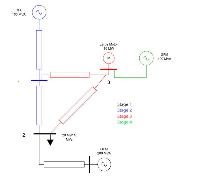
Figure 2 - Test System and Blackstart Stages
6.3. Stage 1
1) Passive Load:
In this step, the GFM plant connects to the load on bus 2, picking up its own transformer, the intermediate transmission line and the load’s transformer in the process. In this scenario, parameter sweeps for the voltage and current controls revealed that the plant is stable for most parameterizations. In the system, a mode that presents oscillations is between the load inductor and the generator. That mode is approximately 59.5 Hz and remains stable but with low damping across most parameter sets. In order to asses the region of stability, a 15 by 15 parameter grid sweep of the voltage controller PI gains is carried out.
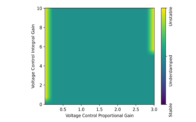
Figure 3 - Voltage Controller Parameter Sweep
The mode in question, presents damping of approximately 4% for low proportional gains of the voltage control. As the proportional gain increases, the mode becomes almost undamped and finally destabilized for large proportional gains, if the integral gain is also tuned to a high value. For parameter sweeps of the current control, for a voltage control proportional gain of 1, the system is stable except for very low proportional gains, although the load mode remains underdamped. There is a well-damped region for low proportional and high integral gains. However, if the proportional gain of the voltage control is tuned to be 2, there exists an unstable region at high integral gains values.
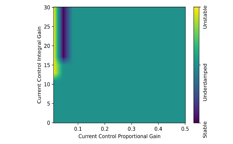
Figure 4 - Current Controller Parameter Sweep
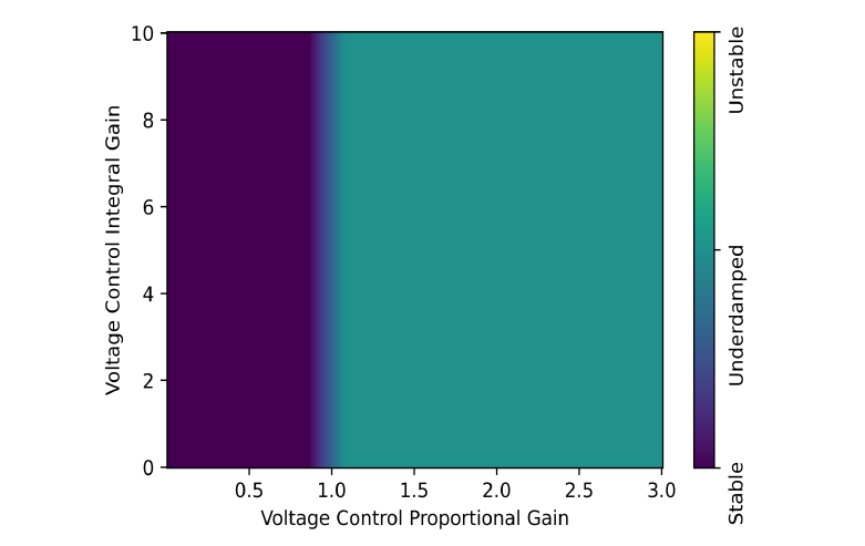
Figure 5 - Voltage Controller Parameter Sweep without Current FF
It should be noted, that across all cases, the instability is extremely slow, as the pole is barely on the right half plane (RHP). In succession, the stability was examined when the current FF gain of the voltage control was disabled (set from 1 to 0), and for that case, the system was stable across all current control parameterizations. For the no FF case, now the system is stable across all PI gains, and low proportional gains seem to offer damping above 5% (below which we deem the mode as under-damped). Thus, this is the trade-off of increasing the voltage control bandwidth and stability. It should be noted, that a parallel RL load is a simple representation of loads that is useful for illustration of the methodology. However, as it will be demonstrated in subsequent sections, the stability of the IBRs will depend on the characteristics of connected load. Alternative representations of RLC loads, inductions motors, inverter-interfaced loads etc. can be expected to yield varying small-signal characteristics. Thus, load modeling is an essential part of accurate dynamic stability assessment.
2) Large Induction Motor:
Next, we examine the GFM stability if the load was a large industrial motor load. Voltage control parameter sweeps indicate that for most parameterizations, there exists an under-damped mode around 54-56 Hz. The mode presents participation from the motor stator fluxes and the inductance of its transformer. In addition, for very low proportional gain values, an unstable mode is captured in the low frequency range (sub 10 Hz). The unstable mode is due to the voltage controller being mistuned. It also presents participation from the motor stator flux states and the current controller integrator state. Finally, in the high proportional gain region, a new instability is observed. Around the value of 2.4, a high frequency mode destabilizes with frequency 252 Hz. The mode presents participation by the motor stator flux states, the GFM LCL circuit currents and voltages, and the GFM voltage transducer state. The GFM voltage transducer cut-off was set to 500 Hz for this test.
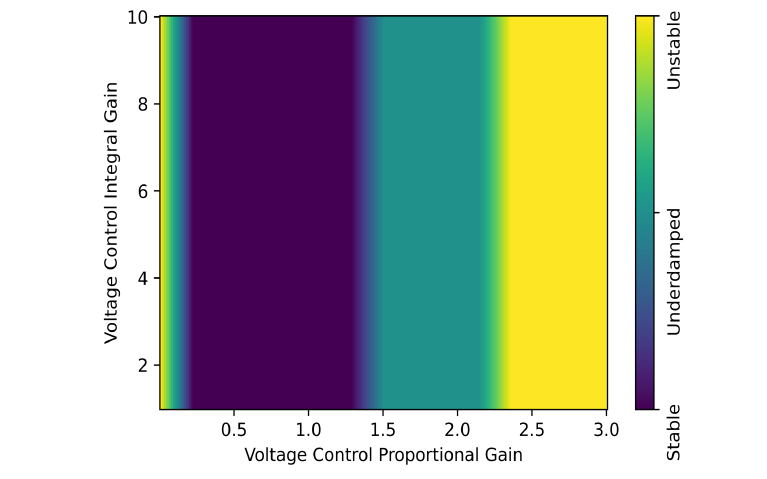
Figure 6 - Voltage Controller Parameter Sweep
The stability was verified with EMT simulations in PSCAD. An example where the proportional gain is ramped from 2 to 2.5 is depicted in Fig. 7. The prediction of the unstable value is close. At 3 seconds, as soon as the gain decreases from the value of 2.5 and crosses 2.4, the mode’s damping increases and the oscillation subsides. The mode frequency was also close to 250 Hz as predicted by our analysis. In addition, the mode frequency appears to be highly dependent on the size of the capacitor present in the motor plant. This dependency was also captured by the participation factor analysis. The capacitor states appear to stop participating significantly when the compensation is reduced to achieve a 0.9 lagging power factor.
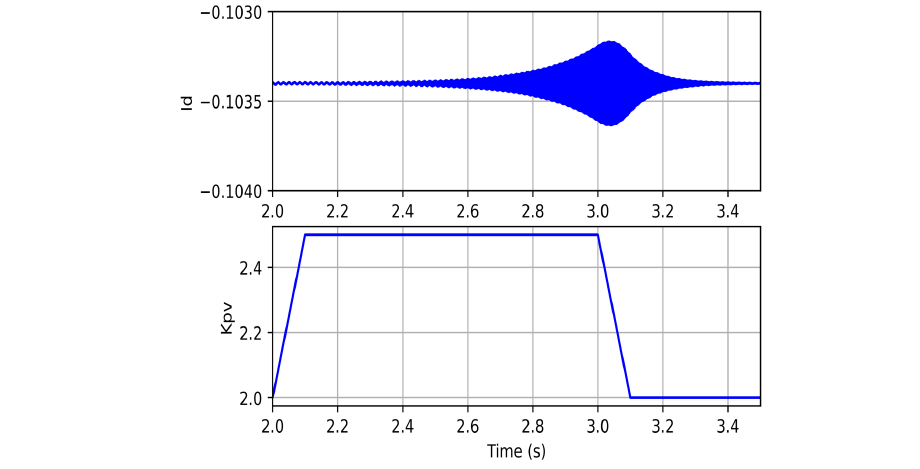
Figure 7 - EMT Simulation for Voltage Control Proportional Gain Ramp
In contrast, if the current FF is disabled for the voltage controller, the high frequency instabilities are no longer observable, and the mode between the GFM and the IM is more well-damped.
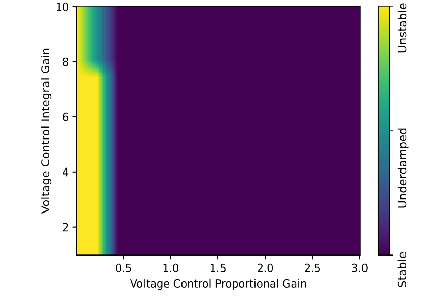
Figure 8 - Voltage Controller Parameter Sweep without FF
When examining the current control tuning, we can note that the mode observed appears to be well-damped for lower proportional gain values. This is to be expected, as lower proportional gains reduce the effective FF gain path for the voltage control output.
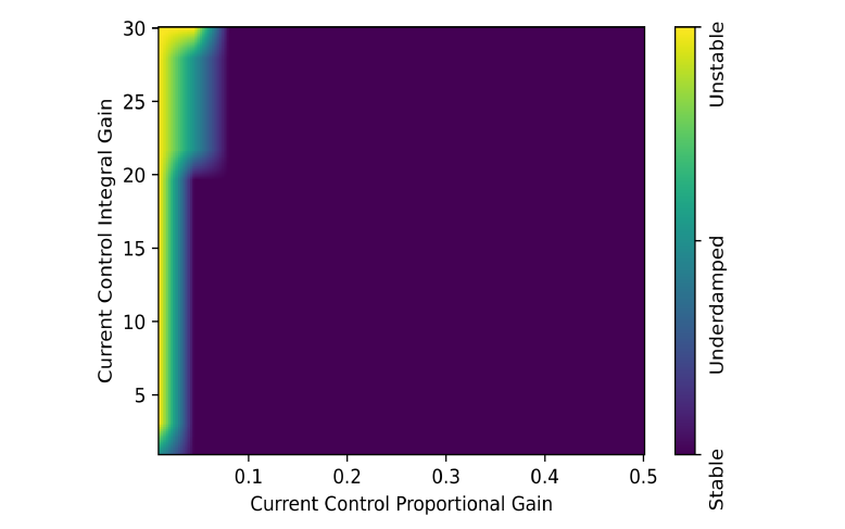
Figure 9 - Current Controller Parameter Sweep
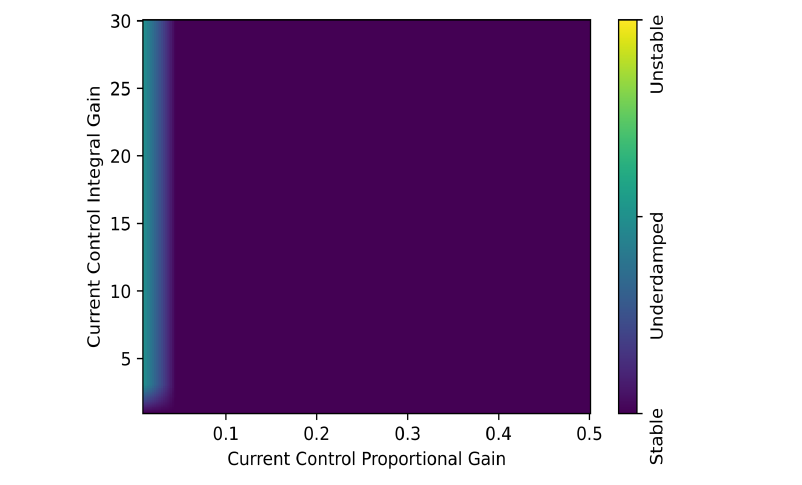
Figure 10 - Current Controller Parameter Sweep without FF
For the subsequent analysis and discussion, the load on bus 2 will be assumed as passive RL.
6.4. Stage 2
In the next step of the energization, a GFL IBR rated at 100 MVA is connected. We examine the stability of the GFL current control when the GFM parameters are fixed. We assume that both plants have a voltage set point of 1 pu, to manage over-voltages when more lines come into the network. As a note, the GFL plant is assumed to offer no frequency control for this analysis. For the initial part of the analysis we shall examine the impact of the GFM tuning on the GFL current parameter sweep. The gains to be altered on the GFM side are the current feed-through F, the current control PI gains and the voltage control PI gains. We shall also examine the impact of voltage set-points and the load type.
Initially, parameter sweeps for the current control parameters of both the GFM and GFL plants were carried out. The mode interacting with the load is still observable. When examining the participation factors, both the GFL and GFM plants appear to contribute. Disabling the current FF (or lowering the gain) can be an effective solution to damp such modes. The no FF cases presented a damping of 4-5%, as seen in Fig. 14, and when the FF was enabled the damping was less than 1%. In general, for most values of current controls the system was stable except for low proportional gains.
The parameter sweeps for the GFM voltage controller revealed more complex stability regions. When FF was enabled, there was a low proportional gain unstable region due to control mistuning. An unstable region for proportional gains of over 2.5 is observed. This corresponds to the destabilization of the GFM - load mode of around 59.5 Hz. When the FF is disabled, the stability of the system is enhanced. The unstable region for high proportional gains is no longer observable. In addition, a high damping region emerges for the GFM/load mode for lower proportional gains. The unstable region at very low proportional gains corresponds to the voltage control loop being unstable, similarly to all the previous parameter sweeps.
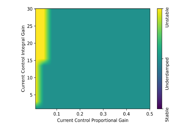
Figure 11 - GFL Current Controller Parameter Sweep
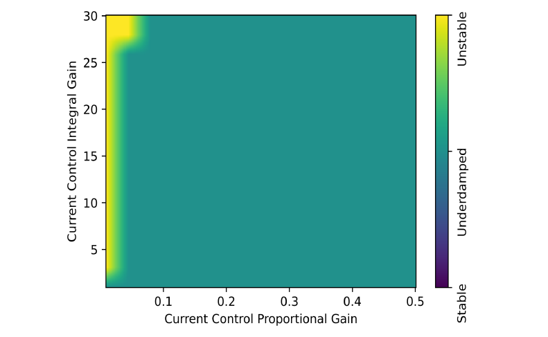
Figure 12 - GFM Current Controller Parameter Sweep
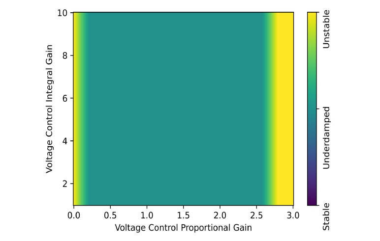
Figure 13 - GFM Voltage Controller Parameter Sweep
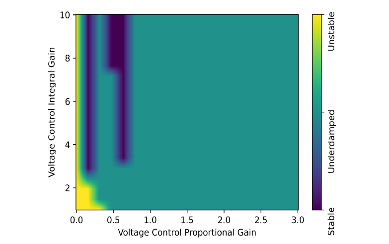
Figure 14 - GFM Voltage Controller Parameter Sweep without FF
In all the studies until now, the plant controller of the GFL IBR was emulated via a first order transfer function. In order to asses how a more realistic approximation of the delay affects stability, the first order transfer function is replaced by a 5th order Pad´e approximation. In this stage, the delay approximation did slightly affect the stability regions of the controls but did not yield significant differences.
6.5. Stage 3
In the next stage the 15 MW large motor load will be connected to the system via two transmission paths. The inertia constant of the motor is assumed to be 1.5. The voltage and current control stability remained consistent similar to the investigations of the previous sections. However, the introduction of a Pad´e approximation for the plant control delay yielded significant variation to the stability of the system. The issues were mainly identified when the current FF of the GFM voltage controller was disabled. For the current controls no new unstable regions were observable, with a small enlargement of the unstable area for low proportional gains when no FF is used. However, for the voltage control, there was a significant difference in the stability region. As noted in Fig. 15 there exists an unstable region for low proportional gains, where the GFL plant control and the motor participate. This region shrinks as integral gains increase. Thus, as the voltage control of the GFM plant gets faster (either through higher gains or FF), the mode is stabilized. We verified the marginally unstable case through EMT simulation, as noted in Fig. 16. The integral gain was tuned to 3 and the proportional gain initially was 2. At around 4.5, the gain is decreased to 0.4 s, driving the system unstable. The mode of approximately 1 Hz, as predicted by our small-signal analysis, slowly increases in amplitude and goes unstable.
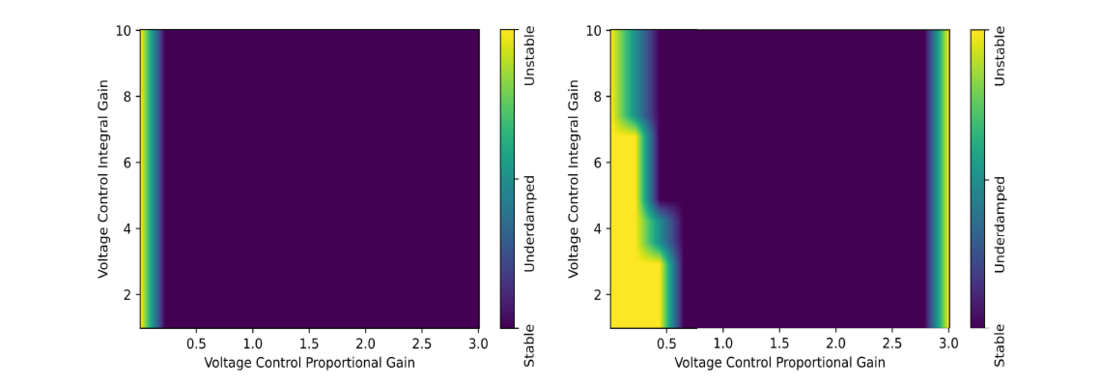
Figure 15 - Voltage Control PI Gains Parameter Sweep (poles below 300 r/s considered). With FF (Left) and no FF (Right)
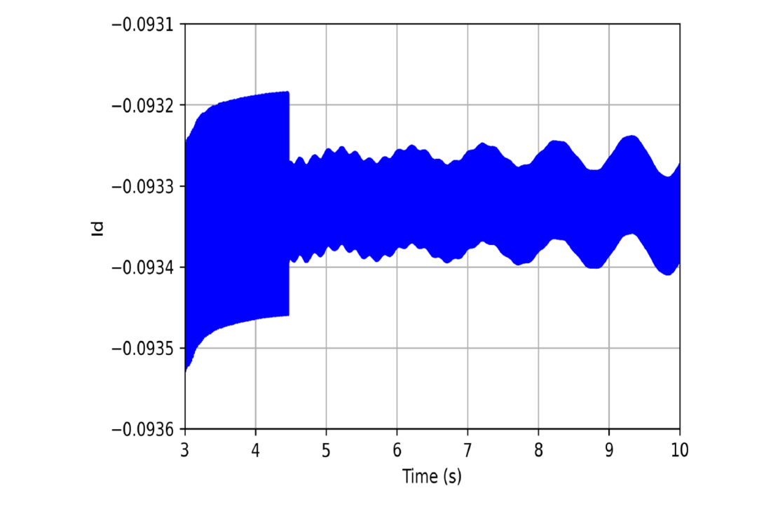
Figure 16 - GFM Voltage Controller d-axis Output with Proportional Gain decrease from 2 to 0.4
We then perform a parameter sweep for the GFL droop gain vs the rating of the motor (motor assumed operating at full load in each scenario) to capture its impact on the unstable mode. For the base case the system remains well damped. However, as the time constant of the GFM P-f droop increases, interactions can be observed between the IBR and the load. The mode of interest is a low frequency mode that is observed between the motor, the GFL voltage controller and reactive power loops and the GFM voltage controller. It is observed to be highly dependent on the size of the motor, the proportional gain of the GFM voltage control and the size of the GFL IBR.
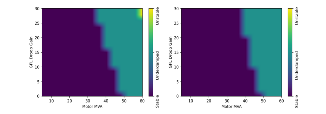
Figure 17 - GFL Droop Gain vs Motor Rating (poles below 100 r/s considered) for GFM Droop Time Constant of 0.1 s (left)) and Time Constant of 0.2 s (right)
For higher motor ratings the mode tends to reduce in damping, especially for higher droop gains. If the current FF is enabled or the proportional gain of the GFM voltage control is tuned higher (without current FF), the mode tends to remain stable. Thus, if we consider a situation were lower proportional gain and no FF is used to avoid exciting the mode observed in Stage 2, the danger of operating in low damping conditions increases if the motor load connected is underestimated.
In order to test the limitations of the GFM to support a GFL plant with aggressive voltage controls, and transfer delays modeled, the GFL plant capacity is doubled (transformer scaled appropriately). The sweep is repeated, revealing that the system now presents instabilities across the majority of the considered cases.
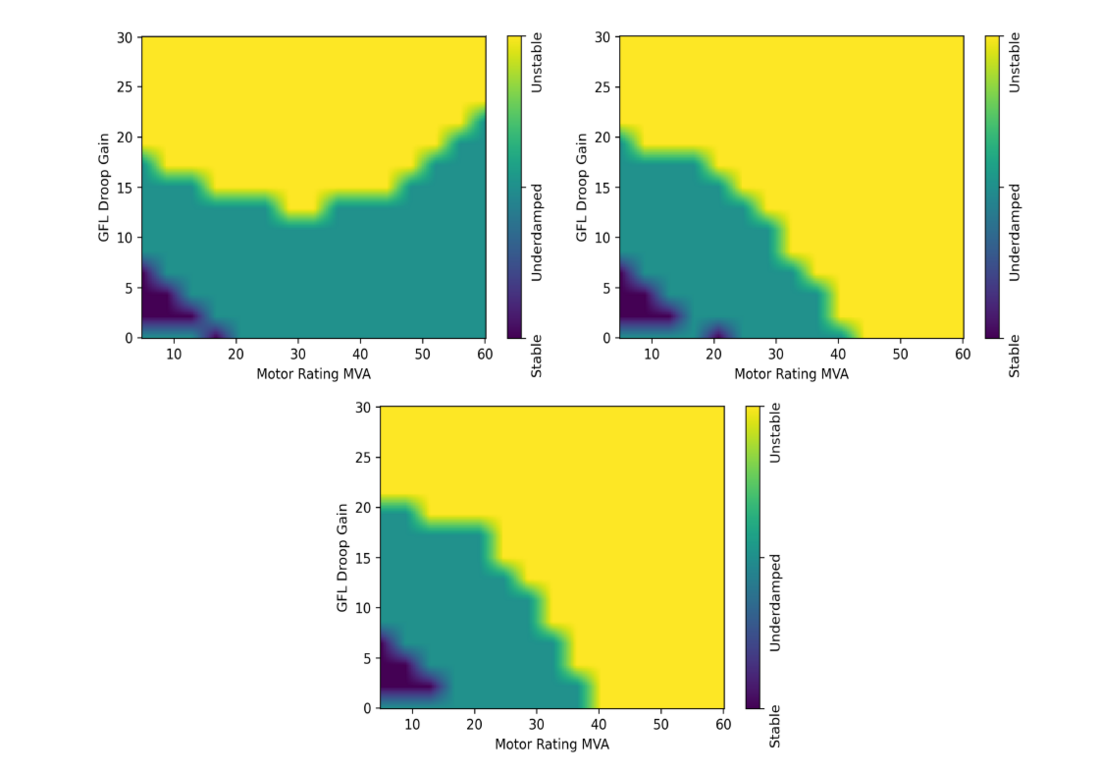
Figure 18 - GFL Droop Gain vs Motor Rating for 200 MVA GFL IBR(poles below 100 r/s considered). Droop Time Constant 10 ms (top left), 100 ms (top right) and 200 ms (bottom)
While keeping the GFL converter at 200 MVA, we now begin to vary the passive load on Bus 2 from 5 to 50 MW (motor is fixed at 15 MW and loading is split between GFM and GFL plants), to identify if there exists a dependence of the motor - GFL - GFM mode on the loading condition of the system, aside from the IM. As it can be noted below, the increase in load offers stabilization to the mode.
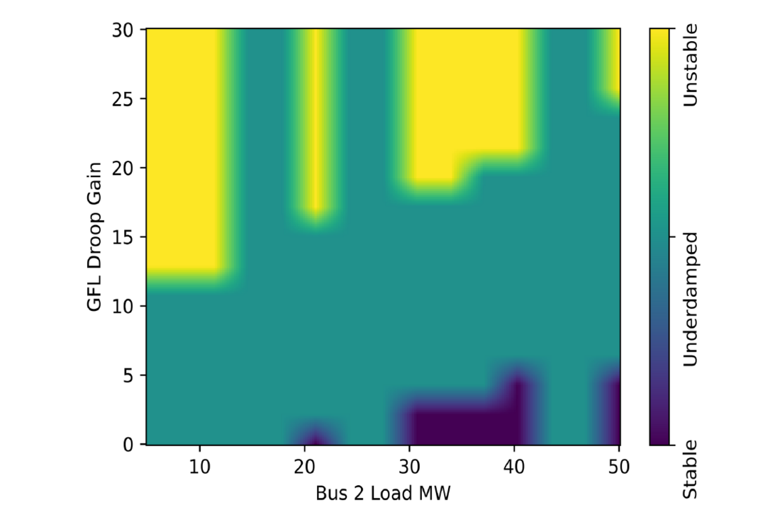
Figure 19 - GFL Droop Gain vs Bus 2 Passive Load for 200 MVA GFL IBR(poles below 100 r/s considered)
It should be noted that given the dependence of the mode on the motor parameters, one should expect different stability characteristics for motors representing different loads (e.g., small industrial or residential motors). Thus, modeling of the load can play a significant role in correctly assessing stability and establishing a BS plan. In addition, given that the root cause of the instability is voltage control interactions with the motor load, lower integral gain of the GFL plant control also leads to stabilization of the mode.

6.6. Stage 4
In the final stage of the system energization, a second 100 MVA GFM IBR connects to the network. The second GFM connects at the motor bus via its own transformer. In this new stage, a new mode of interest can be observed. The mode of instability is around 30 Hz. The participating IBRs are the two GFM plants. The mode observed to have high sensitivity to the voltage control gains of the GFM plants, the use of current feed-through and DC boost converter gains. Voltage control parameter sweeps for GFM 2 were carried out under varying droop gains (same for both GFM plants). Increases in droop gains are associated with smaller stable regions of the system.
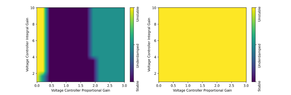
Figure 20 - Voltage Control Parameter Sweep of GFM 2 for various P/f Droop Gains Applied to Both GFM Plants (poles below 300 r/s) 2% (Left) and 5% (Right)
For the droop time constant, we can note a significant stabilization as time constants increase. This can be attributed to the droop loop becoming slower, thus not interacting with the voltage and current controls as much, hence not destabilizing the system. For the FF gain, values over 0.96 appeared to destabilize the system. This was observed for the 5% droop case. As noted in Fig. 21, as soon as the value crosses 0.96 oscillations start growing and the system quickly starts to destabilize as the gain increases to 1. As soon as the value decreases below 0.96 the mode appears to improve in damping. For the lower droop case, this instability was not observed.
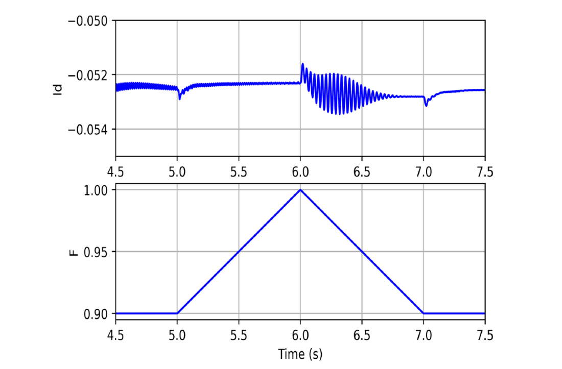
Figure 21 - Varying GFM 1 Current FF Gain Instability
As mentioned, the unstable mode is also highly dependent on the parameterization of the DC boost controller. In the base case, the boost control was tuned to be fast, with PI gains of 1/10. We retune to more moderate gains of 0.2/5 and scan again the voltage control stability region (FF remains enabled). As noted in Fig. 22, the system now has a large region of stability for all modes below 300 r/s, which are well-damped.
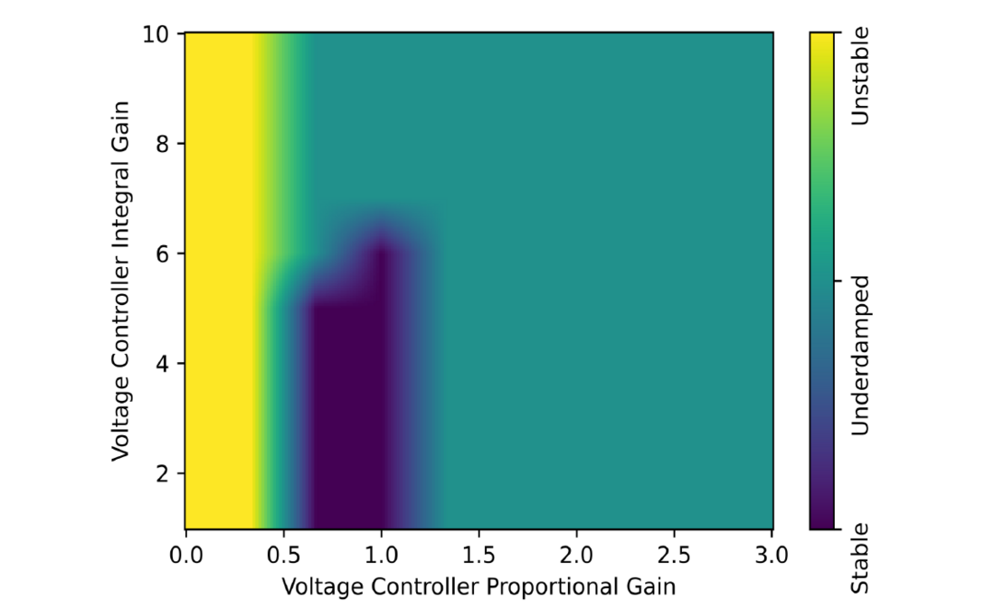
Figure 22 - Voltage Control Parameter Sweep of GFM 2 for Moderate DC Boost Control Gains(poles below 300 r/s)
Finally, the parameter sweep for the current control reveals that for high integral gains, the control is unstable across all proportional gains.
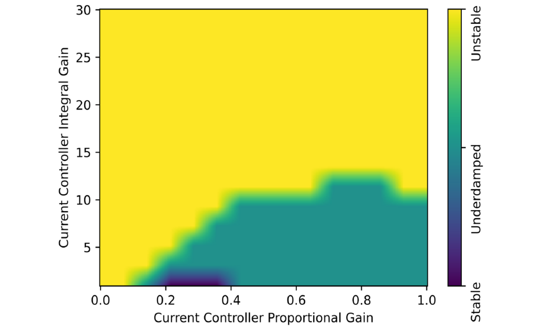
Figure 23 - Current Control Parameter Sweep of GFM 2 (poles below 300 r/s)
For lower DC boost control gains, we can once again note an enlargement of the stability region.
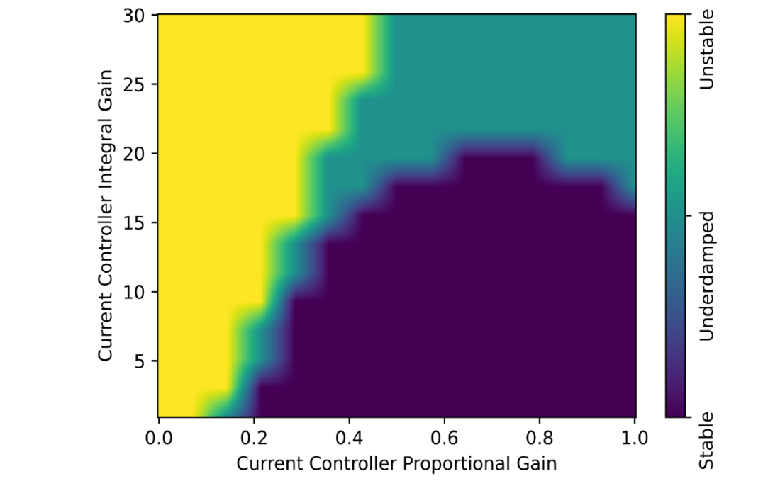
Figure 24 - Current Control Parameter Sweep of GFM 2 for Moderate DC Boost Control Gains(poles below 300 r/s)
7. Conclusion
This work has revealed that during a blackstart procedure, the dynamics of the online network change drastically as the load and generation mix changes in each stage. It is paramount that operators can ensure the stability of the system during these early stages of restoration, as the dynamics can be fundamentally different than when the whole system is connected. We have demonstrated that IBRs can be smallsignal stable during a 100% renewable-based blackstart process. However, the dynamics and stability can be challenging to asses without exhaustive EMT simulations. Small-signal analysis methodologies, such as the process described in our work, can be a valuable tool for operations engineers, needing to assess system stability, and if needed, examine alternative IBR tuning or energization order if the established blackstart plans prove to have poor stability properties.
For Stage 1, the phenomena of interest when the loads were modeled as RL circuits, were for under-damped modes around 59 Hz. The modes were stable but worsened in damping with higher proportional gain of voltage controls. If the load was modeled as a large motor, the mode of interest was at 252 Hz, destabilized by very high proportional gains of the voltage control. Moderate gains of the voltage control, or reduction of the current FF gains of the voltage control can alleviate those issues.
In Stage 2, the load was an RL circuit, thus the mode was still observable. Now new significant instabilities were observed with the introduction of the GFL plant. Transfer delays of the plant control did not appear to affect the stability as well.
In Stage 3, a large IM was connected to the “live” network via two transmission paths. In this stage, a new mode between the motor flux states and the GFL/GFM voltage controls manifests. As GFL plant size increases the mode destabilizes more. In addition, if the GFL plant is assumed to offer fast frequency response, the droop gain tuning can be a highly sensitive parameter as it pertains to stability. Only moderate gains were observed to be stable. The situation is also exacerbated if the P-f droop time constant of the GFM plant increases. The mode was also found to be dependent on the IM parameters. As expected, when frequency response of GFL plant is enabled in such small networks, care should be exercised in the tuning of gains and the response time of the droop loops. Also, the GFL plant size played a role in stability. Thus, one should consider the amount of GFM capacity present in the energized network and how introduction of GFL plants can effect the voltage controller stability and the system’s frequency response.
In Stage 4, a second GFM plant was introduced. The system became unstable for the base parameterization used up until that stage. The mode of interest concerned the voltage controllers of the two GFM plants. The mode was highly sensitive to the PI gains of the controls, the use or not of current FF and the PI gains of the DC voltage boost control.
It should be noted that the instabilities observed can vary based on modeling of components, parameterization, order of energization and the amount of load connected. Our work aims to highlight the wide array of dynamic characteristics a power system during blackstart can occupy, especially when the process is based on IBRs. Our future work aims to expand our analysis to target other renewable resources and the role they can play in blackstart, while analyzing their dynamic characteristics and interactions with other IBRs and loads, including converter controlled loads.
Finally, an important aspect of high-penetration IBR networks that requires further investigation, is in regards to the amount of GFM MVA required to support GFL plants in a blackstart setting. As noted in the results of Stage 3, voltage control interactions can occur when the GFM/GFL mix was 50/50 and the GFL plant employed high voltage control gains and plant control transfer delays were approximated by the Pad´e approximation.
It should be noted, that this work aims to outline a procedure that can be utilized by engineers to screen for small-signal stability, when establishing a BS plan. Varying topology, load/generator types and operating conditions, can significantly alter small-signal behavior. As a result, this work aims to demonstrate the methodology rather than try to derive an “optimal” set of parameters for this particular system or make any broader conclusions about specific parameterization or control structures. Furthermore, if the goal is to evaluate stability for multiple loading conditions for the same topology, they can be screened in parallel to establish the system’s small-signal stability robustness towards load variation. For large disturbances, such as significant load steps, large-signal evaluations such as time domain simulations are required, as the assumption of linearity no longer holds for the examined dynamics of the system.
8. Appendix
PV Plant
| Element | Value | Unit |
|---|---|---|
| Rd | 1.51158 | Ω |
| Ld | 0.44828 | mH |
| Cd | 196.19 | μF |
| Lf1 | 0.044828 | mH |
| Lf2 | 0.044828 | mH |
| Cf | 392.39 | μF |
| CDC | 10000 | μF |
Base IBR Parameters
GFM Converter:
| Controller | Prop. Gain | Int. Gain |
|---|---|---|
| Voltage Control | 1 | 10 |
| Current Control | 0.5 | 20 |
| DC Voltage Boost Control | 1 | 10 |
| Controller | Gain | Time Constant |
|---|---|---|
| Active Power | 0.05 | 0.01 |
| Reactive Power | 0.05 | 0.01 |
| Parameter | Value |
|---|---|
| DQ Voltage Transducer Time Constant | 3.183 10-4 |
| DQ Current Transducer Time Constant | 1.591 10-4 |
| Current FF Gain | 1 |
GFL Converter:
| Controller | Prop. Gain | Int. Gain |
|---|---|---|
| Voltage Control | 2 | 20 |
| Current Control | 0.5 | 20 |
| Active Power Regulator | 0.1 | 10 |
| Reactive Power Regulator | 1 | 10 |
| PLL | 50 | 700 |
| DC Voltage Boost Control | 1 | 10 |
| Active Power Droop | 0 | 0 |
| Parameter | Value |
|---|---|
| DQ Voltage Transducer Time Constant | 3.183 10-4 |
| DQ Current Transducer Time Constant | 1.591 10-4 |
| Terminal Voltage Transducer Time Constant | 0.02 |
| Active Power Transducer Time Constant | 0.02 |
| Reactive Power Transducer Time Constant | 0.02 |
| GFL Plant Controller Delay Time Constant | 0.15 |
Network Data
| Element | R | X | B |
|---|---|---|---|
| GFM 1 Transformer | 0 | 0.05 | 0 |
| GFM 2 Transformer | 0 | 0.1 | 0 |
| GFL Transformer | 0 | 0.1 | 0 |
| Line GFM 1 | 0.002655 | 0.046192 | 0.20184 |
| Line GFL | 0.00177 | 0.03082 | 0.1345 |
| Line 1-2 | 0.00177 | 0.03082 | 0.1345 |
| Line 2-3 | 0.001065 | 0.0185 | 0.0806 |
| Line 1-3 | 0.0027 | 0.0474 | 0.2072 |
Induction Motor Data
The motors used in this work utilize the parameters from [22]. The motors are assumed to operate at 100% loading. Motor loading variation (80-100%) did not yield significant results to the small-signal stability properties of the system.
References
- R. Henriquez-Auba, J. D. Lara, C. Roberts and D. S. Callaway, “Grid Forming Inverter Small Signal Stability: Examining Role of Line and Voltage Dynamics,” IECON 2020 The 46th Annual Conference of the IEEE Industrial Electronics Society, Singapore, 2020, pp. 4063-4068, doi: 10.1109/IECON43393.2020.9255030.
- W. Du et al., “A Comparative Study of Two Widely Used Grid-Forming Droop Controls on Microgrid Small-Signal Stability,” in IEEE Journal of Emerging and Selected Topics in Power Electronics, vol. 8, no. 2, pp. 963-975, June 2020, doi: 10.1109/JESTPE.2019.2942491.
- L. Ding, X. Lu and J. Tan, “Comparative Small-Signal Stability Analysis of Grid-Forming and Grid-Following Inverters in Low-Inertia Power Systems,” IECON 2021 – 47th Annual Conference of the IEEE Industrial Electronics Society, Toronto, ON, Canada, 2021, pp. 1-6, doi: 10.1109/IECON48115.2021.9589651.
- L. Ding, X. Lu and J. Tan, ”Small-Signal Stability Analysis of Low- Inertia Power Grids with Inverter-Based Resources and Synchronous Condensers,” 2022 IEEE Power & Energy Society Innovative Smart Grid Technologies Conference (ISGT), New Orleans, LA, USA, 2022, pp. 1-5
- R. Henriquez-Auba, J. D. Lara, C. Roberts and D. S. Callaway, “Grid Forming Inverter Small Signal Stability: Examining Role of Line and Voltage Dynamics,” IECON 2020 The 46th Annual Conference of the IEEE Industrial Electronics Society, Singapore, 2020, pp. 4063-4068, doi: 10.1109/IECON43393.2020.9255030.
- S. Shah, P. Koralewicz, V. Gevorgian, H. Liu and J. Fu, ”Impedance Methods for Analyzing Stability Impacts of Inverter-Based Resources: Stability Analysis Tools for Modern Power Systems,” in IEEE Electrification Magazine, vol. 9, no. 1, pp. 53-65, March 2021.
- C. Zhang, M. Molinas, A. Rygg and X. Cai, ”Impedance-Based Analysis of Interconnected Power Electronics Systems: Impedance Network Modeling and Comparative Studies of Stability Criteria,” in IEEE Journal of Emerging and Selected Topics in Power Electronics, vol. 8, no. 3, pp. 2520-2533, Sept. 2020
- Y. Liao and X. Wang, ”Impedance-Based Stability Analysis for Interconnected Converter Systems With Open-Loop RHP Poles,” in IEEE Transactions on Power Electronics, vol. 35, no. 4, pp. 4388-4397, April 2020
- Ye, Mao, et al. ”Security margin analysis of wind power participating in black start.” The Journal of Engineering 2019.18 (2019): 5214-5218.
- M. Rasheduzzaman, J. A. Mueller and J. W. Kimball, ”Reduced-Order Small-Signal Model of Microgrid Systems,” in IEEE Transactions on Sustainable Energy, vol. 6, no. 4, pp. 1292-1305, Oct. 2015, doi: 10.1109/TSTE.2015.2433177.
- L. Fan and Z. Miao, “A Modular Small-Signal Analysis Framework for Inverter Penetrated Power Grids: Measurement, Assembling, Aggregation, and Stability Assessment”, arXiv:2003.03860.
- S. Konstantinopoulos, D. Ramasubramanian, E. Farantatos and V. Singhvi, “Blackstart and Restoration of 100% Renewable Power Systems with Grid Forming Converters,” 2022 IEEE Power & Energy Society General Meeting (PESGM), Denver, CO, USA, 2022, pp. 1-5, doi: 10.1109/PESGM48719.2022.9916718.
- Q. Nguyen, M. R. Vallem, B. Vyakaranam, A. Tbaileh, X. Ke and N. Samaan, “Control and Simulation of a Grid-Forming Inverter for Hybrid PV-Battery Plants in Power System Black Start,” 2021 IEEE Power & Energy Society General Meeting (PESGM), Washington, DC, USA, 2021, pp. 1-5, doi: 10.1109/PESGM46819.2021.9637882.
- H. Jain, G. -S. Seo, E. Lockhart, V. Gevorgian and B. Kroposki, “Blackstart of Power Grids with Inverter-Based Resources,” 2020 IEEE Power & Energy Society General Meeting (PESGM), Montreal, QC, Canada, 2020, pp. 1-5
- S. Thakar, S. Konstantinopoulos, V. Verma, D. Ramasubramanian, M. Bello, J. Xu, J. Mesbah, W. Zhou, and B. Bahrani (2024) Topic 2 – Analytical methods for determination of stable operation of IBRs in a future power system. CSIRO, Australia.
- PSCAD Knowledge Base: Simple Solar Farm, Available online
- Yazdani, Amirnaser, and Reza Iravani. Voltage-sourced converters in power systems: modeling, control, and applications. John Wiley & Sons, 2010.
- C. Yang, L. Huang, H. Xin and P. Ju, “Placing Grid-Forming Converters to Enhance Small Signal Stability of PLL-Integrated Power Systems,” in IEEE Transactions on Power Systems, vol. 36, no. 4, pp. 3563-3573, July 2021, doi: 10.1109/TPWRS.2020.3042741.
- L. Fan, Z. Miao, D. Ramasubramanian and H. Ding, “Operational Challenges of Solar PV Plus Storage Power Plants and Modeling Recommendations,” in IEEE Open Access Journal of Power and Energy, vol. 10, pp. 477-489, 2023.
- Belikov, J., Levron, Y. Integration of long transmission lines in largescale dq0 dynamic models. Electr. Eng. 100, 1219–1228 (2018). https://doi.org/10.1007/s00202-017-0582-7
- P. Kundur, Power System Stability and Control. New York, NY, USA: McGraw-Hill, 1994.
- L. Pereira, D. Kosterev, P. Mackin, D. Davies, J. Undrill and Wenchun Zhu, “An interim dynamic induction motor model for stability studies in the WSCC,” in IEEE Transactions on Power Systems, vol. 17, no. 4, pp. 1108-1115, Nov. 2002, doi: 10.1109/TPWRS.2002.804960.