Grid-Forming and Grid-Following inverters: a dynamic performance evaluation using RMS, EMT and small-signal analysis
Authors
Luis David PABО́N OSPINA- Fraunhofer IEE
Deepak RAMASUBRAMANIAN - Electric Power Research Institute

Summary
The dynamic performance of inverter-based resources is of increasing importance in power system dynamics. Over the past decade, new types of instabilities driven by inverter controls have emerged, leading to the need for stability studies using the two main types of inverter control: Grid-forming and Grid-following controls. However, there exists a widespread misconception, prevalent across industry, research, and academia, that Grid-following control is inherently “bad” while Grid-forming control is universally “good.” This research challenges this misconception by demonstrating the evaluation of inverter controls based on their performance rather than the internal controller architecture. Through comprehensive time-domain RMS, EMT, and small-signal analysis, this study demonstrates that properly tuned Grid-following inverters can exhibit comparable performance to Grid-forming inverters across a wide range of operational conditions. Additionally, the paper addresses the limitations of each technology, particularly in extreme weak grid scenarios.
Keywords
Dynamic performance, Grid-Forming inverter, Grid-Following inverter, Power system stability, Small-signal stability1. Introduction
Recently, there have been numerous publications highlighting instabilities caused by inverter controls, which were not common in traditional power systems with large Synchronous Generators (SGs). But these stability concerns have been reported in literature and real-world operations for over a decade. Many of these instabilities have been referred to as Converter-Driven Instability (CDI) following the definition provided by [1]. CDI has gained significant attention due to its manifestation as undamped voltage and power oscillations in real-world operations in the presence of Inverter-Based Resources (IBRs). The dynamics of the Phase-Lock Loop (PLL) have been identified as one of the major contributors to this phenomenon, particularly in weak grid operating conditions [2]. This has influenced the perception of power engineers towards Grid-Following (GFL) inverter control, as it requires the utilization of a PLL for network synchronization.
On the other hand, Grid-Forming (GFM) inverters may not require a PLL for network synchronization. This feature, combined with other advantageous control characteristics, can make GFM inverters a highly appealing solution, particularly for weak networks. This paradigm shift in inverter controls has contributed to the notion that GFL is inherently “bad” while GFM is universally regarded as “good”.
In this paper, the term GFL refers to a range of inverters with varying capabilities, from injecting power at unity power factor without grid services to advanced inverters offering voltage and frequency support, relying on a PLL for network synchronization. On the other hand, GFM refers to inverters providing grid services, capable of withstanding load-generation mismatch and potentially enabling black start capability, without requiring a PLL for network synchronization.
1.1. Understanding the negative perception that power engineers have of Grid-Following Inverters
Several works have conducted studies on oscillations that are triggered by GFL inverters. A comprehensive survey of real-world subsynchronous oscillation events associated with IBRs is presented in [3], providing a list of real-world cases between 2007 and 2023, mostly attributed to PLL dynamics during weak grid conditions. A study conducted in the Manitoba Hydro system, [4], uncovered oscillations with frequencies around 8 Hz that are influenced by controller gains and effective short circuit ratio (ESCR) at the inverter bus. The influence of weak grids, characterized by a low Short Circuit Ratio (SCR), and PLL parameters on the dynamic behavior of a HVDC converter is examined in [2], demonstrating the significant impact of PLL gains, particularly at low SCRs, on the operation of the HVDC converter. Moreover, the study highlights the challenges associated with operating at low SCRs approaching 1.3, indicating the difficulties involved in such scenarios as instabilities may arise. An example of subsynchronous oscillations in distribution grids is provided in [5] through small-signal and RMS simulations, highlighting that the stability concern also extends to Distribution System Operators (DSOs). In this case, a French DSO investigates potential slow-interaction CDI caused by GFL control with high-gain PLL. The possibility of oscillations caused by GFL controls resulting from reduced system strength due to unstable long-term dynamics is examined in [6]. The study concludes that even with careful tuning for both pre- and post-contingency scenarios, GFL inverters continue to be susceptible to oscillations if the long-term dynamics result in a weaker system with SCR values that push GFL control to its limitations. This finding implies that traditional countermeasures against long-term instability or collapse may be compromised in their effectiveness if GFL controls oscillate. Reference [7] makes a strong statement, pointing out that GFL-IBRs do not contribute to system strength like SGs but instead have the overall effect of reducing it.
1.2. Understanding the Positive Perception that power engineers have of Grid-Forming Inverters
GFM technology as the potential key for high IBR penetration is investigated in [7]. The dynamics of a network that consists of 100% IBRs with both GFM and GFL inverters are analyzed by the authors in [8]. The study reveals that as the number of GFM inverters increases, a quicker recovery is observed following a fault event. Additionally, the presence of more GFM inverters in the transmission network leads to tighter voltage and frequency levels. A comparison of GFL and GFM controls, specifically focusing on Fault Ride Through (FRT) assessment in weak grids, is conducted in [9]. The findings suggest that with GFL control, significant frequency variations are observed, while GFM control is deemed more suitable for operation in weak grid conditions. The dynamic performance of GFL and GFM for frequency support in low inertia grids is evaluated in [10]. The case study indicates that while the GFL control with frequency-real power droop can achieve a similar frequency nadir as the GFM methods, it tends to exhibit higher Rate of Change of Frequency (RoCoF) and a smaller transient stability margin. The limitations of commonly used GFL, including inadequate grid support capability and low stability, are highlighted in [11]. In response, emerging GFM control methods have been proposed to enhance the dynamic performance and stability. The findings suggest that GFL control exhibits poor stability and dynamic performance due to its current source characteristics. In contrast, GFM control shows promise as a grid-friendly alternative, capable of functioning as a voltage source to provide grid support. Various stability issues arising due to GFL-IBRs losing stability with low system strength are stated in a study performed for the Queensland transmission network, [12]. The use of GFM is considered to be one promising solution for system strength issues. Reference [13] proposes the utilization of GFM batteries to suppress oscillations that may arise from the interaction between GFL controlled type-4 wind farms and weak ac networks.
2. Discussion and contributions of this paper
Given this context, it is understandable that a common misconception exists where GFL control is often perceived as inherently “bad” while GFM control is seen as universally “good.” However, most of the above-mentioned conclusions are obtained by comparing GFM with GFL controls that: 1) were tuned for strong grids, but not properly tuned for weak grid conditions, and 2) do not provide voltage and frequency response but rather only provide active and reactive power control. There are few publications such as [14], in which the authors conduct a fair comparison between both technologies. The study sheds light on the fact that both control methods can be prone to instability if not appropriately designed. It emphasizes that control design and tuning are equally crucial for achieving optimal performance in both GFL and GFM inverters. Another example is illustrated in [15], which states that GFM devices require an appropriate control setup and should not be assumed to be plug-and-play components. With simulations conducted on the Australian National Electricity Market (NEM) network, it demonstrates that poorly tuned GFM control has a negative influence on system damping and can be more destabilizing than having no inverter at all. By using a wide-area EMT model, the Australian Electricity Market Operator (AEMO) showed in [15] that GFM Virtual Synchronous Generator (VSG) settings chosen without consideration of the existing system have the potential to exacerbate existing oscillatory instabilities. The simulations conclude that better system-wide damping can only be achieved with careful consideration of the electrical location of the IBR, as well as the settings of the IBR controllers, regardless of the IBR technology.
This paper shows, without neglecting the limitations, that:
- Properly tuned GFL-IBRs can perform comparably to GFM-IBRs across a wide range of operational conditions.
- Poorly damped oscillations in extreme low SCR cases cannot be attributed solely to GFL controls.
- Well-tuned GFL controls exhibit high damping ratios for PLL-related oscillation modes even at extremely low SCR.
- Oscillation modes with low damping may involve contributions from states within SG controls, and the frequency of oscillation may resemble electromechanical oscillations rather than converter-driven oscillations.
- GFM controls can also exhibit oscillatory behavior under low SCR conditions and may pose stability concerns. Careful considerations are also necessary for GFM controls in weak systems.
- The difference between well-tuned GFL and well-tuned GFM controls becomes evident only at very low SCR values (e.g., below 1.2), where GFM control demonstrates better performance. More importantly, even for these cases, small -signal analysis confirms that oscillations cannot be attributed solely to GFL controls.
- The stability and reliability of a future high-IBR power system should not rely solely on GFM-IBRs. Instead, responsibility should be shared among different technologies, including GFL-IBRs, to ensure high reliability.
3. Test System and IBR Models
The IEEE Nordic test system is depicted in Figure 1, focusing on the Central region. In this region, a SG has been replaced with an IBR. For detailed information about the system and its controllers, please refer to [16] and [17]. The test system can be downloaded from the IEEE Power System Dynamic Performance Committee website [18] in various formats. It is worth noting that the Central zone is characterized by relative weakness, with substantially more load than available generation capacity. By replacing only one SG in this area with an IBR, SCRs as low as 1.0 are easy to achieve, even in the base case without contingency, while considering realistic rated powers of utility-scale IBRs. As will be demonstrated later, the SCR value decreases significantly in the event of line openings due to system faults. This makes the substitution of one SG with an IBR suitable for the conducted studies.
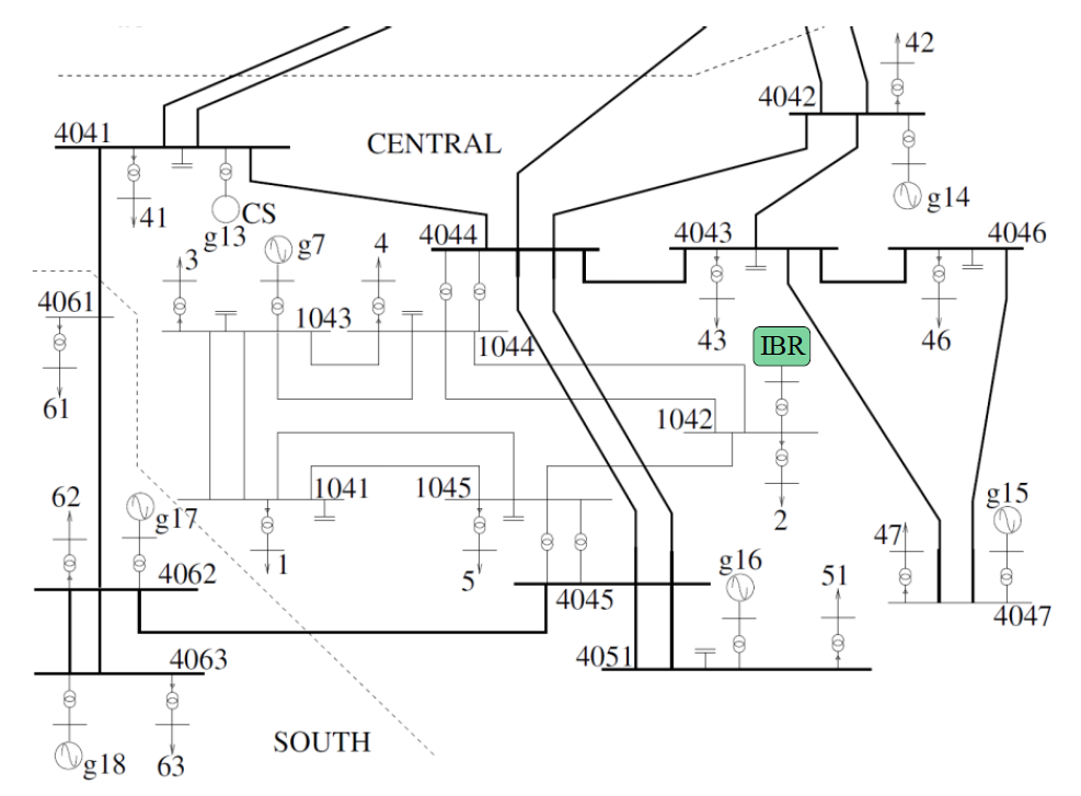
Figure 1 - Central zone - IEEE test system for voltage stab. assessment [16], [17]
Standardized models available in commercial software tools have been employed for the IBRs. Specific references are provided for each model to avoid redundant descriptions in this paper. However, it is important to highlight certain key aspects, which are summarized as follows:
3.1. WECC large-scale IBR model
Details can be found in [19], [20], [21], [22]. Of particular relevance to the studies conducted in this work is the voltage interface with the network solution, as shown in Figure 2.
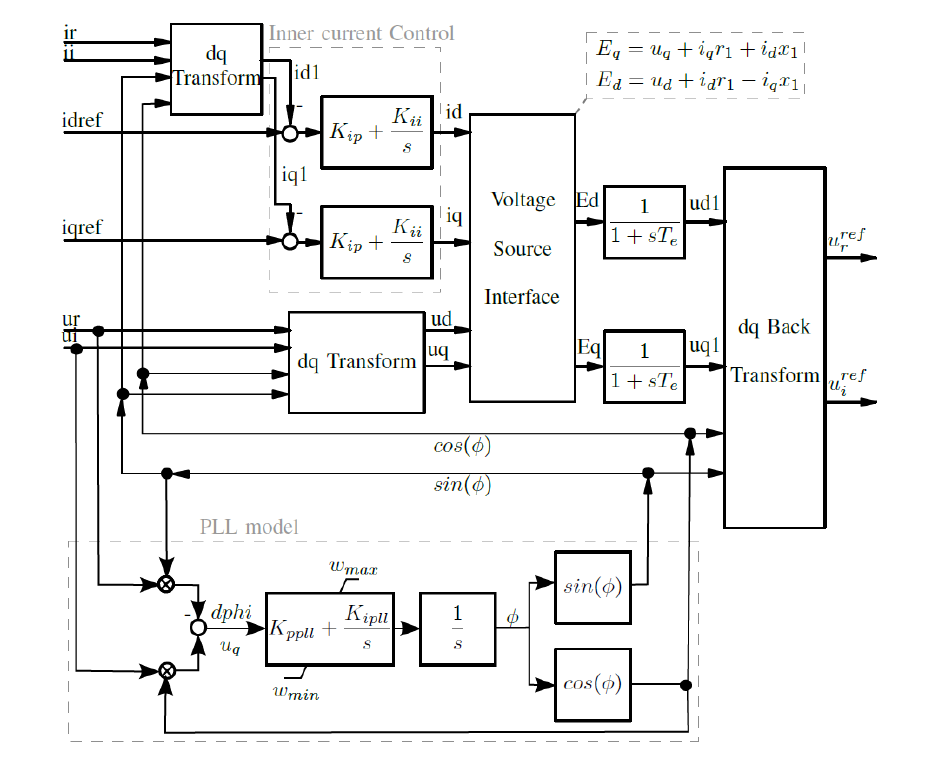
Figure 2 - IBR voltage source interface, inner control and PLL [6], [19]-[22]
These models have been developed and validated by members of the WECC Model Validation Subcommittee (MVS). The plant control is based on the REPC_A model, while the outer control relies on REEC_B [23], [24]. The generator control, represented by REGC_C, includes a simple PLL and inner current control, as demonstrated in Figure 2. The signals ????? and ????? come from the outer control, in this case REEC_B. The model is used for RMS simulations.
3.2. GFM Virtual Synchronous Machine (VSM)
Details can be found in [25], [26]. The complete model comprises current and voltage measurements, a power calculation block, a grid-forming controller (with the actual VSM), a virtual impedance block, a voltage controller, and an output voltage calculation block. Of particular relevance to the studies conducted in this work is the actual VSM (Figure 3) that emulates the mechanical part of a synchronous machine, which is also referred to as the swing equation.
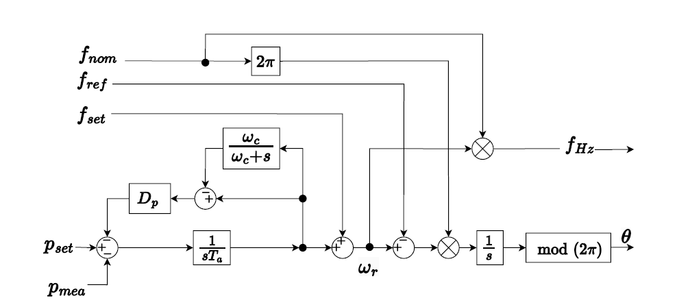
Figure 3 - Simplified VSM model
A VSM can be represented by the approximated synchronous machine per unit balance in the Laplace domain according to the following equation [27]:
(1)
?? represents the mechanical time constant, ???? denotes the active power setpoint, and ???? represents the measured active power output. The rotating speed of the VSM is denoted by ??. Additionally, ???? refers to the frequency setpoint, and ?? represents the damping coefficient. The input ???? (in p.u.) in Figure 3 represents the reference frequency in RMS simulations. It can be set to the nominal frequency (constant throughout the simulation and equal to 1 p.u.) or to the calculated center of inertia. The input ???? (in p.u.) is the frequency setpoint for the GFM model (equivalent to ???? in (1), as it is also in p.u.). It is initialized with the same value as ????; if initialized with a different value, it will modify the droop equation accordingly. As mentioned in [25], this model is applicable for both RMS and EMT simulations, with specific considerations that are taken into account during initialization.
3.3. GFM Droop control
Details can be found in [25], [28]. It reuses all the blocks of the VSM model, but the grid-forming control block is replaced by the droop control. In this case, the following equations are employed.
(2)
?? and ?? represent the active and reactive power droop coefficients. ????? and ????? denote the low-pass filtered active and reactive power deviations from the load flow initialization, respectively. As mentioned in [25], this model is applicable for both RMS and EMT simulations, with specific considerations that are taken into account during initialization.
3.4. EMT Models
In practice, GFL control typically includes outer loops, such as power controls, which provide references to the current loops. However, these outer loops can also introduce negative damping effects, particularly under weak grid conditions. The EMT models used in this work consider all these components to capture potential instabilities caused by different controls. Detailed PLL, outer control, inner current control loop, and voltage-source interface (Figure 4) are explicitly modeled. Details can be found in [29]. Of particular relevance to the studies conducted in this work is the more detailed PLL models that can be either a synchronous reference frame (SRF) PLL with notch filters, or a decoupled double synchronous reference frame (DDSRF) PLL. An example is shown in Figure 5. Details can be found in [30], [31].
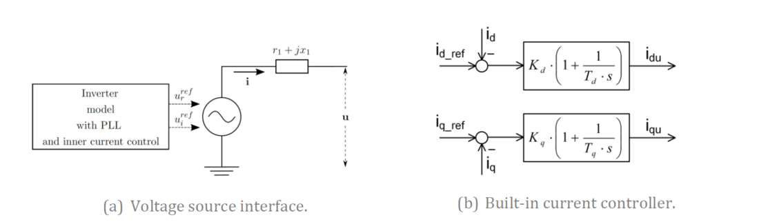
Figure 4 - Built-in voltage source and current controller [29]
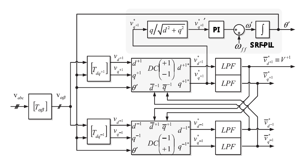
Figure 5 - Structure of the DDSRF-PLL [30], [31]
3.5. Modes in the original system
Table 1 presents critical and lightly damped modes from the original test system to aid in analyzing the interaction between the system modes and the modes of the IBRs. Only modes with damping ratio below 10% are presented.
| Real Part [1/s] | Imaginary Part [rad/s] | Damped Frequency [Hz] | Damping Ratio [%] |
|---|---|---|---|
| -0.352 | ± 6.168 | 0.982 | 5.692 |
| -0.417 | ± 5.866 | 0.934 | 7.098 |
| -0.519 | ± 7.161 | 1.140 | 7.233 |
| -0.280 | ± 3.385 | 0.539 | 8.258 |
| -0.596 | ± 6.844 | 1.089 | 8.676 |
| -0.728 | ± 7.707 | 1.227 | 9.407 |
| -0.723 | ± 7.519 | 1.197 | 9.566 |
| -0.837 | ± 8.263 | 1.315 | 10.042 |
As anticipated for the original system, which consists solely of synchronous generators, the damped frequencies do not exceed a few Hertz. In fact, most are around 1 Hz, which is typical of electromechanical oscillations.
Participation factor analysis reveals that the mode with the lowest damping is strongly influenced by the state variables corresponding to the speeds of generators g15 and g06, both located in the critical area.
4. Small-signal analysis of the PLL subsystem
Let us start the analysis by linearizing the PLL and computing its frequency response. As a concept-friendly example, the state-space representation of the PLL in Figure 2 is given by [6]:
(3)
where the inputs u=[?? ??] are the real and imaginary components of the measured voltage. The state ?2 is the estimated terminal voltage phase ?. The outputs sin(?2) and cos(?2) are used in the direct-quadrature-zero transformation. The state ?1 is the one associated with the PI controller. The equilibrium points can be found solving ẋ = f(x∗,u∗) = 0 for the state-space equations in (3). Hence, the set of equilibrium points for an input
are given by:
(4)
where:
(5)
As can be deduced from (5), the system has multiple equilibrium points, which is a common characteristic of nonlinear systems. Linearizing according to the initial values of ?? and ?? which are the result of an initial load flow, the following eigenvalues are obtained (the mathematical derivations are presented in Appendix A):
(6)
Note that ?ppll and ?ipll are positive parameters. Therefore, when ? is odd, the left part of (6) is greater or equal to zero. In such a case, the point is always unstable as there will be at least one eigenvalue in the positive real part of the complex plane.
5. Study case with SCR = 3.35 and high-gain PLL
In this case, the IBR in the Central zone has a nominal power of 300 MVA. The resulting SCR is 3.35 for the base case without contingency. As will be shown later, this value decreases significantly in the post-contingency scenario, particularly in the event of line openings due to system faults. Let us start with a case in which the PLL gains are set to ?ppll=10 and ?ipll=2000. The voltage at the IBR terminals is |u∗|=1.01 ??.
5.1. Analysis of the linearized PLL
The Bode plot of the linearized PLL is shown in Figure 6. In this case, the bandwidth is 11 Hz and it is the result of PLL gains inside typical ranges.
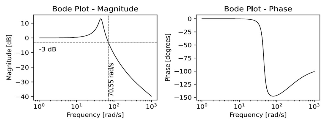
Figure 6 - Bode plot of linearized PLL - bandwidth = 11 Hz
It is worth noting that the magnitude plot exhibits a significant peak at a natural frequency of approximately 44 rad/s, where the phase crosses -90 degrees. This observation suggests the presence of an oscillation mode within the subsystem with relatively low damping at this specific frequency (7.1 Hz). To visually represent this phenomenon, refer to Figure 7. In this figure, the grey plane defined by the real and imaginary axis is the same plane typically used to visualize eigenvalues in small-signal studies. The figure illustrates the Bode magnitude plot alongside the eigenvalues of the matrix ?. Only the eigenvalue with a positive imaginary part is depicted (green point), given the logarithmic scale. As anticipated based on replacing the values of ?ppll, ?ipll and |u∗| (with ?=0) in equation (6), the PLL contributes to an oscillation mode characterized by ? = −5.05 ± 44.659?. This aligns with the observed peak at approximately 44 rad/s in the Bode magnitude plot.
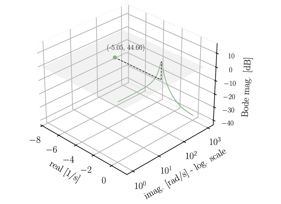
Figure 7 - Bode plot and eigenvalues of linearized PLL - bandwidth = 11 Hz
5.2. Small-signal analysis for the entire system
Figure 7 depicts the frequency response and eigenvalues of a specific subsystem, namely the PLL. However, to gain a broader understanding of the system behavior, it is necessary to compute the eigenvalues of the entire system. In this case, the small-signal analysis function of a commercial software tool is employed to obtain the results displayed in Figure 8.
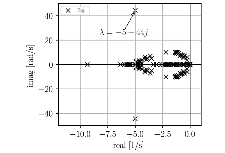
Figure 8 - Eigenvalues of the entire system (PLL-bw = 11 Hz)
Figure 9 facilitates the comparison between the previous analysis on the linearized PLL and the eigenvalues of the entire system. In this figure, the eigenvalues of the entire system are represented by black markers. They are overlaid with the eigenvalues and Bode plot resulting from the PLL analysis, represented by the green point and the green line respectively.
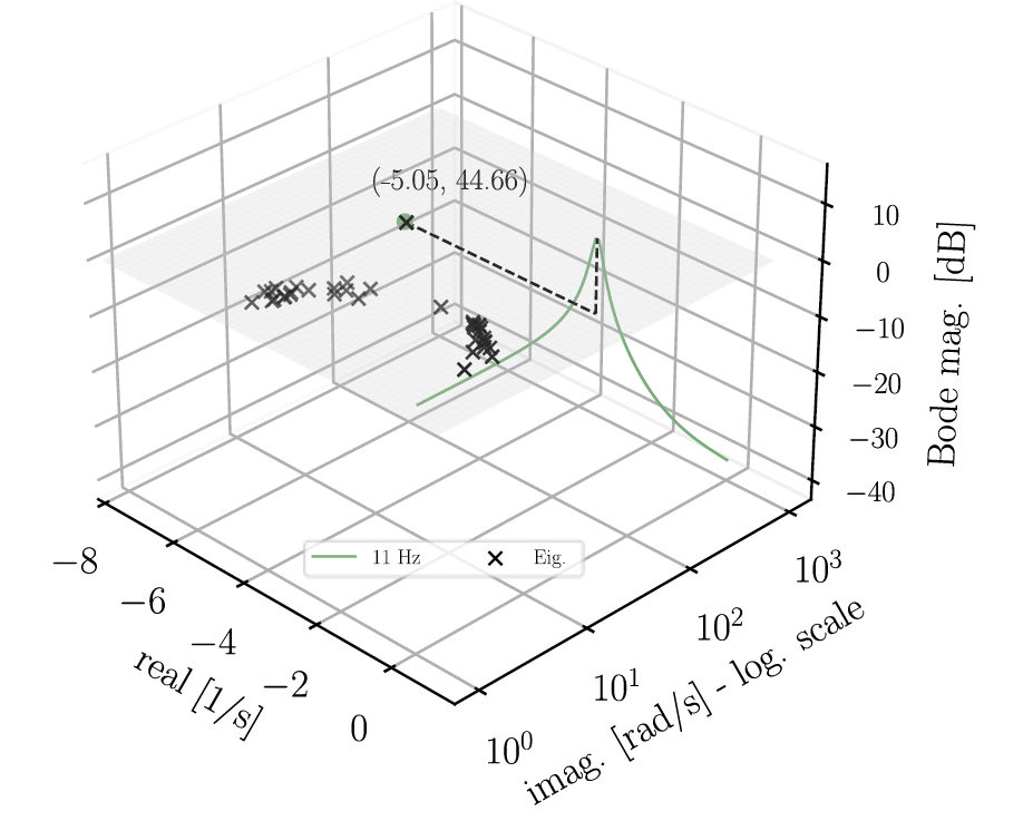
Figure 9 - Bode plot of linearized PLL and eigenvalues of the entire system - PLL bandwidth = 11 Hz
The results obtained from both the small-signal analysis of the entire system and the linearized PLL analysis demonstrate a high correlation. This correlation confirms the presence of an oscillation mode at the natural frequency where the Bode magnitude exhibits a significant peak. Furthermore, a participation factor analysis verifies that this mode is indeed influenced by the PLL states. In this specific case, the participation factor analysis indicates that the PLL state variables are the only ones contributing significantly to this mode. However, it is important to note that in some cases, additional states may also have considerable participation in such a mode. As a result, the mode may shift from what would be initially concluded by analyzing only the PLL subsystem.
5.3. Time-domain analysis
In this case, a three-phase short circuit is simulated at 95% of one of the lines 1044-1042. It is important to note that the fault occurs in close proximity to bus 1042, where the IBR is connected. The short circuit is cleared after 100 ms with no line reclosure. Figure 10 shows the EMT simulation results.
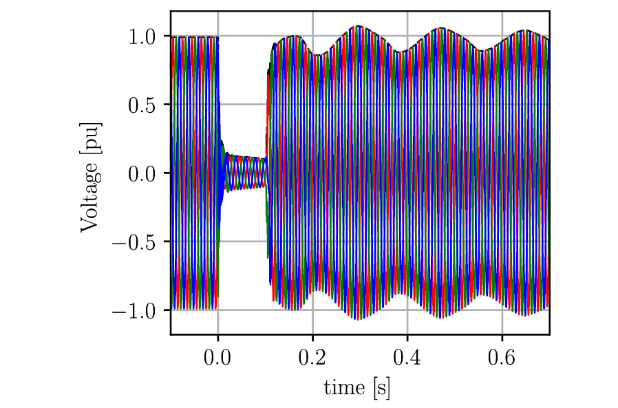
Figure 10 - EMT results - Phase voltages at bus 1042 - PLL bandwidth = 11 Hz
Since there is no line reclosure, the post-contingency SCR drops significantly to approximately 2.2. The presence of oscillations after the fault clearance is evident.
To further analyze these oscillations, a Fast Fourier Transform (FFT) is performed on the voltage phasor magnitude (represented by the black envelope in Figure 10). The resulting FFT magnitude is depicted by the blue line in Figure 11.
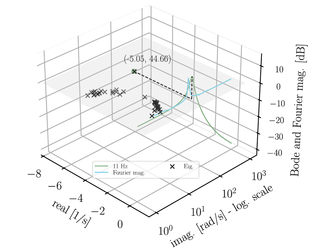
Figure 11 - Bode plot of linearized PLL, eigenvalues of the entire system and Fourier magnitude of
EMT results - PLL bandwidth = 11 Hz
The FFT results indicate a significant component at frequencies near the natural frequency of the PLL and the frequency of the detected oscillation mode from small-signal analysis. To comprehend the strong correlation between these different results, it is crucial to consider the following: 1) The results presented in green represent the linearized version of a single small subsystem, specifically the PLL. 2) The results marked with black markers also originate from a linearized system (small-signal analysis for the entire network). 3) The results displayed in blue correspond to the FFT analysis conducted on the results of an EMT simulation, which considers all non-linearities present in the model. 4) The strong correlation remains consistent even when considering a large disturbance event in the EMT results, as opposed to the small-signal analysis.
5.4. Effect of reducing the PLL bandwidth
Let us now gradually reduce the bandwidth of the PLL while analyzing the impact on the Bode magnitude and small-signal analysis.
Figure 12 displays the response when the PLL bandwidth is reduced to 9 Hz. The previous results are still shown with a grey dashed line for comparison. It is worth noting that the results from the small-signal analysis (black markers) still overlap with the oscillation mode predicted by the linearized PLL analysis (green point), which has the form ? = −5 + 35.8?.
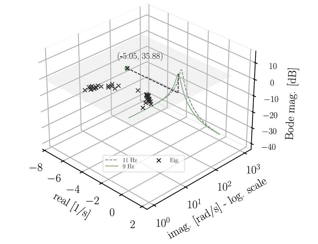
Figure 12 - Bode plot of linearized PLL and eigenvalues of the entire system - PLL bandwidth = 9 Hz
Figure 13 displays the results when the PLL bandwidth is further reduced to 6 Hz. In this case, the Bode magnitude appears to be “flatter”, but there is still an oscillation mode ? = −5 + 21.9? at its natural frequency. The correlation with the small-signal results remains consistent.
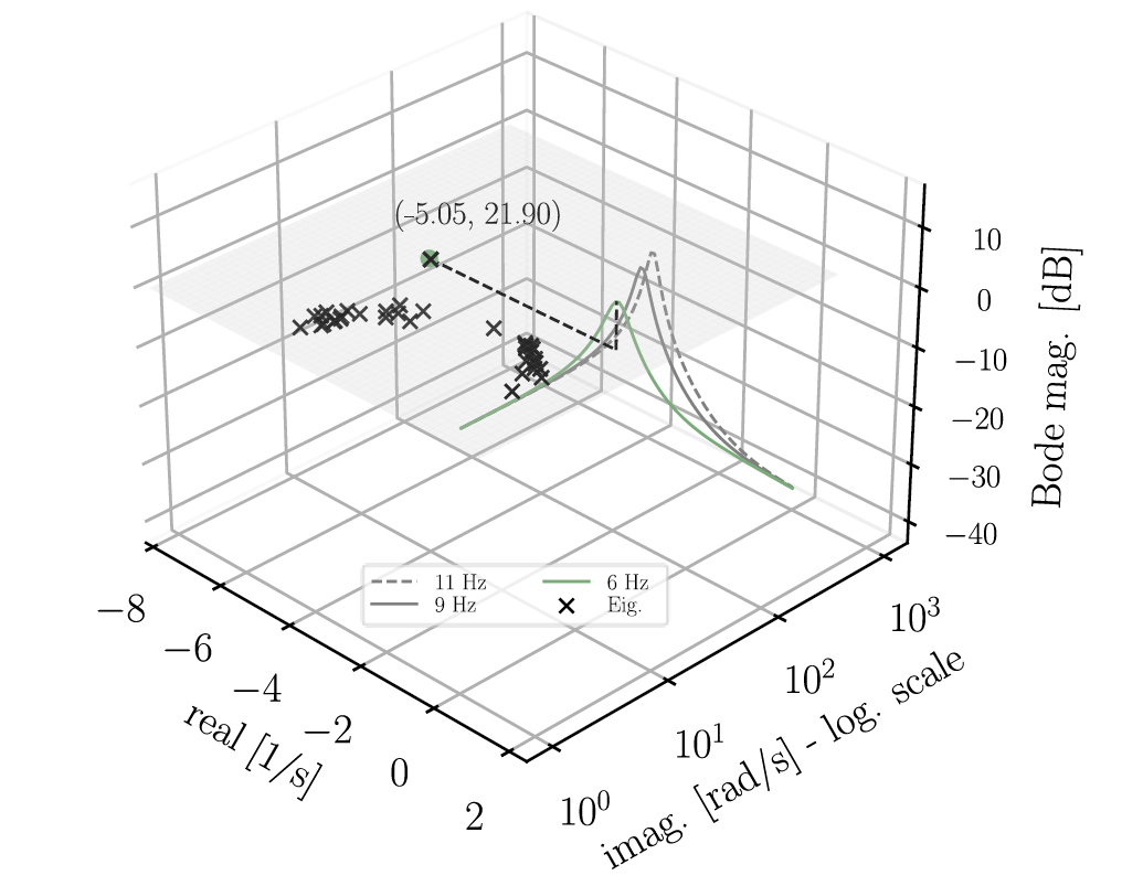
Figure 13 - Bode plot of linearized PLL and eigenvalues of the entire system - PLL bandwidth = 6 Hz
Figure 14 displays the results for a PLL bandwidth of 4 Hz. In this case, the impact of the reduced bandwidth is evident. Not only does it flatten the Bode magnitude, eliminating the peak that occurred at the natural frequency, but it also “removes” the oscillation mode that was highly influenced by the PLL states and caused undamped oscillations (observed in Figure 10). Note that the oscillation mode that is highly influenced by the PLL states does not actually “disappear.”
Instead, it ``moves”, as demonstrated in the next section.
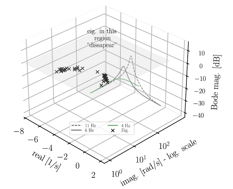
Figure 14 - Bode plot of linearized PLL and eigenvalues of the entire system - PLL bandwidth = 4 Hz
For the sake of completeness, the effects of reducing PLL bandwidth are further confirmed by the time-domain simulations shown in Figure 15. These simulations consider two additional bandwidth values, namely 8.2 Hz and 7.9 Hz. The simulation results align with all conclusions previously drawn from EMT and small-signal analysis. Specifically, a properly tuned GFL inverter can perform effectively in low SCR scenarios. However, it is important to note that this comes with certain limitations, which will be discussed later.
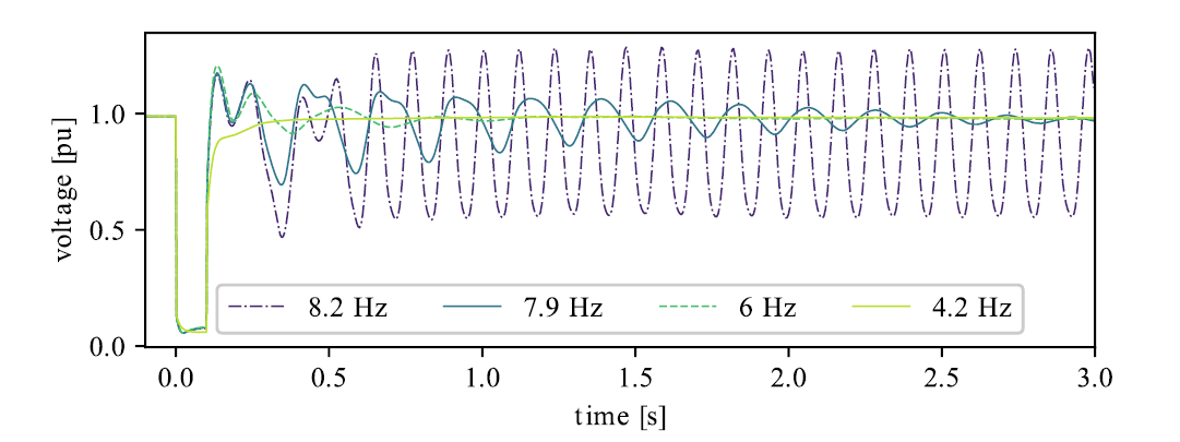
Figure 15 - RMS results - different PLL bandwidth
The analysis indicates that a lower PLL bandwidth enhances system stability, particularly in weak grid conditions. However, this improvement in stability comes at the cost of response speed: a lower PLL bandwidth leads to slower reactions to changes in grid conditions and setpoint adjustments. It is crucial to verify dynamic performance against specific grid code requirements, such as FRT and maximum rise time after setpoint adaptation. This presents a trade-off between stability and the inverter's dynamic performance in terms of response speed. In this case, the simulation results demonstrate effective voltage recovery and do not indicate any potential violations of grid code requirements, such as FRT.
5.5. Resemblance of tuned GFL with a GFM control
Since the results in Figure 14 show a significant improvement in the damping of the oscillation mode (which depends on the amplitude of the Bode magnitude at the natural frequency), it is appropriate to compare the small-signal results of this GFL-IBR against a GFM-IBR. In this case, a VSM control is considered and the results are shown in Figure 16.
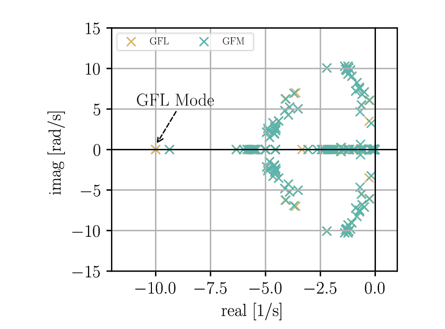
Figure 16 - Eigenvalue comparison GFL (PLL bw = 4 Hz) and GFM-VSM
The resemblance is remarkable, with only a few noticeable differences at first glance. The most significant distinction is the non-oscillatory mode characterized by ? = −10 ± 0?. Participation factor analysis confirms that this mode is influenced by the PLL state variables of the GFL-IBR. This initial insight given by the small-signal analysis results suggests that well-tuned GFL inverters can achieve comparable performance to GFM-IBRs under certain scenarios. This assertion is further supported by Figure 17, which illustrates the similarities in the EMT simulation results. It is worth highlighting that the SCR after the line trip is 2.2, which is deemed as a low value. Nevertheless, the GFL control still performs effectively.
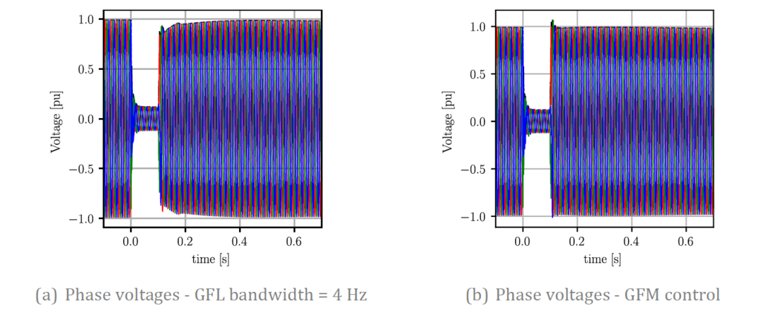
Figure 17 - Comparison of EMT results between GFL and GFM
6. Study cases with lower SCR scenarios
6.1. Limitations of bandwidth tuning
The previous results were obtained for an operating scenario with an SCR of 3.35 (2.2 after the line trips), which is critically low. However, in some exceptional situations, the SCR in real systems can be lower. To investigate the effects of reduced SCR, Figure 18 presents the EMT results for GFL with 4 Hz bandwidth and different SCR cases. Please note that the SCR values described in Figure 18 correspond to the pre-contingency operating point. This means that once the line is
tripped, the SCR will decrease further. Note that in this study case, critically low SCR values, such as 1.2, necessitate large utility-scale IBRs. In this instance, the nominal power is 800 MVA, which, although high, remains within realistic ranges.
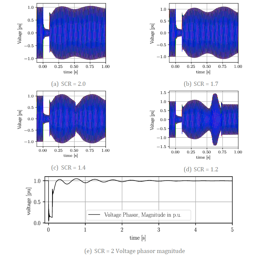
Figure 18 - Comparison of EMT results for GFL - Different SCR
The results demonstrate the limitations of the reduced-bandwidth approach. As the SCR decreases, oscillations become more apparent. The dynamic performance remains acceptable when the SCR = 2 (1.3 post-contingency), as shown in Figure 18 (a). This is further confirmed by the EMT results depicted in Figure 18 (e), which specifically focuses on the voltage phasor magnitude. The plot reveals well-damped oscillations that decay in about three seconds. Note that the phasor magnitude plot up to five seconds is not necessary for the other SCR cases as they are unstable. The oscillations become increasingly prominent when the SCR is reduced to 1.7 and 1.4. An interesting case arises when the SCR is 1.2, where the oscillations exhibit negative damping. This results in a rapid increase in voltage to very high values for less than 100 ms. Subsequently, a switch-off threshold is reached, causing the IBR to trip shortly before 0.8 s. It is important to emphasize that these limitations are encountered in extreme cases of low SCR, i.e., post-contingency SCR less than
1.1. Similar conclusions can be derived from [32], [33], and [34], which identify 1.2 as a critical SCR value for stable operation of GFL inverters.

6.2. PLL modes for extreme cases of low SCR
As mentioned, the limitations observed in Figure 18 are encountered in extreme cases of low SCR. Specifically, when the line is disconnected, the SCR drops to values as low as 0.86 in Figure 18 (d). Such low SCR values are not only exceptional in bulk power systems but also indicate an atypically weak network. This implies that network reinforcements are necessary, and that the poor dynamic performance is not solely attributed to oscillations caused by GFL control. To investigate this, Figure 19 shows the small-signal results for different cases of post-contingency SCR. This means that the eigenvalues are calculated in the new steady state without one of the lines 1044-1042. Different PLL bandwidths are considered for each SCR.
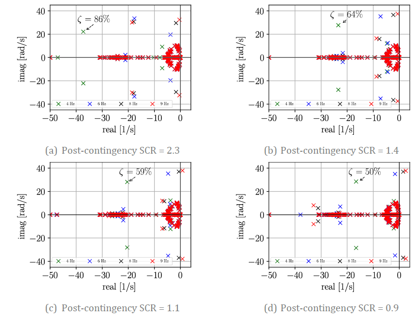
Figure 19 - Eigenvalues for GFL and different post-contingency SCR
Let us start by analyzing the case with a PLL bandwidth of 9 Hz (red markers). When the SCR is 2.3, the oscillation mode influenced by the PLL exhibits very low damping. With an SCR of 1.4, the mode is almost marginally stable. When the SCR is 1.1, the oscillation mode displays negative damping. In this scenario, the oscillations are clearly attributed to the unstable mode and it can be concluded that the observed oscillations are caused by GFL control, and more precisely, by the PLL dynamics. A similar situation occurs with a PLL bandwidth of 8 Hz (black markers).
The situation undergoes a change when the PLL bandwidth is set to 6 Hz, as indicated by the blue markers. It is worth noting that even with a post-disturbance SCR of 0.9, as shown in Figure 19 (d), the oscillation mode remains in the left semi-plane, albeit very close to the imaginary axis. This indicates a low damping characteristic, suggesting that the poorly damped oscillations could potentially be attributed to the dynamics of the GFL control and PLL.
The situation significantly changes when the PLL bandwidth is set to 4 Hz (green markers). The damping ratio for different SCR cases has been highlighted. For instance, when the post-contingency SCR is 2.3, the damping ratio is ? = 86%. Even with a decrease in SCR to 0.9, the damping ratio of the PLL mode remains ? = 50%. In power system dynamics, a damping ratio of at least 10% is generally considered indicative of a “well-damped” mode [35]. Comparing this threshold, the PLL oscillation mode with a damping ratio of ? = 50% is very well-damped. Consequently, it can be concluded that the observed oscillations cannot be directly attributed to the GFL control or PLL dynamics in this case. A damping ratio of 50% clearly signifies a well-damped mode; however, it is important to avoid generalizing the need for damping ratio thresholds exceeding 10%. The simulations conducted in this study do not seek to establish the minimum pre-contingency damping ratio required to ensure well-damped oscillations across all credible contingencies. In accordance with NERC recommendations in [36], simulation studies should be undertaken to assess how contingencies impact a mode's damping ratio, thereby informing the selection of suitable damping ratio thresholds. However, this aspect falls outside the scope of the current work.
Furthermore, there are modes with low damping ratio that could lead to the oscillations seen in Figure 18. For instance, when the post-contingency SCR is 1.1, the mode with the lowest damping ratio has the form ? = −0.33 ± 6.19?, resulting in ? = 5.36%, which is considered low. Participation factor analysis reveals that several state variables contribute to this mode, all belonging to synchronous generators, including generators in the Central zone such as g15 and g16. This mode exhibits a damped frequency of 0.98 Hz, which is typical of electromechanical oscillations and not indicative of oscillations caused by inverter control. In fact, the observed oscillations in Figure 18 also exhibit frequencies that are typical of electromechanical oscillations, around 2 Hz in this case.
Moreover, under extremely low SCR conditions, oscillatory behavior can occur with GFM control as well. This can be illustrated by referring to Figure 20, which presents the EMT results using a GFM control with VSM. The results show that, just as in the case of GFL control, if the GFM-IBR is not properly tuned, oscillatory behavior is plausible.
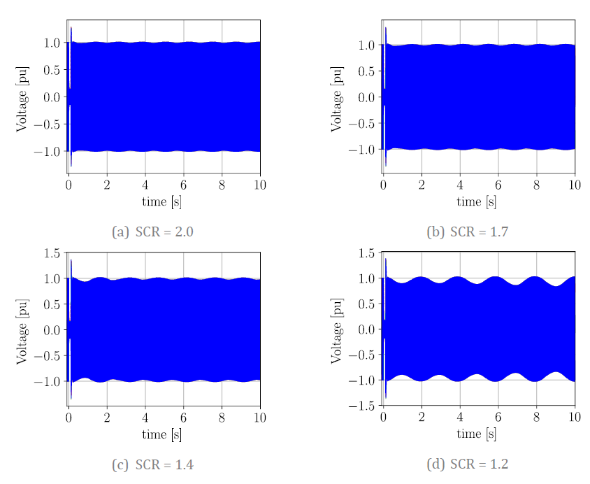
Figure 20 - Comparison of EMT results for poorly tuned GFM - Different SCR
The same conclusion is supported by small-signal analysis. Let us consider the case illustrated in Figure 20-d. The eigenvalues of the system are presented in Figure 21-a, where a mode with negative damping (-0.03 1/s) is identified. Participation factor analysis indicates that the unstable mode is primarily influenced by the state variables associated with the first-order block (1/??? ) and the pure integrator shown in Figure 3.
As the damping coefficient increases from 3 to 10, the unstable mode shifts to the left half-plane, and no oscillatory modes are observed in Figure 21-b, even under extremely low SCR conditions. It is important to note that this work does not focus on optimal parameter tuning, and the specified values will vary based on system characteristics. The purpose of this analysis is to demonstrate that even with a GFM control, parameter values can significantly impact system stability.
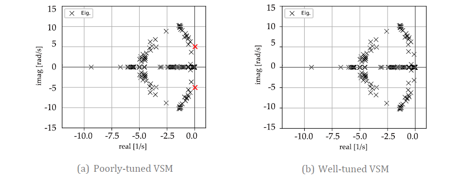
Figure 21 - Comparison of eigenvalue results for poorly- and well-tuned GFM
These results are not meant to imply that GFM control cannot contribute to improving the dynamic performance observed in Figure 18 and Figure 20. Instead, they are meant to emphasize that GFL control is not necessarily the one to be held responsible for oscillatory behavior. In contrast, Figure 22 shows the response with a properly tuned GFM control. It is evident that the GFM control can operate stably for lower SCR conditions, but as long as the GFL-IBRs are properly tuned, the difference starts being evident at exceptionally low values (e.g., SCR around 1.0 after the contingency). Even in such cases, the observed oscillations cannot directly be attributed to GFL control, as concluded by the small-signal analysis.
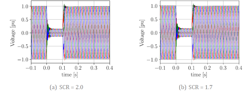
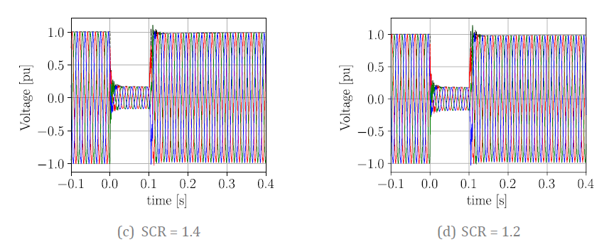
Figure 22 - EMT results for properly tuned GFM - Different SCR
7. Conclusions
This work challenges the misconception that GFL is inherently “bad” while GFM is universally “good.” Through time-domain and small-signal analysis, it is confirmed that GFL controls are not solely responsible for poorly damped oscillations, even under extreme low SCR scenarios. When GFL controls are properly tuned, even at post-contingency SCR levels as low as 0.9, the PLL-related oscillation modes exhibit high damping ratios of up to 50%, indicating well-damped modes. This demonstrates that properly tuned GFL control cannot be directly attributed to the observed oscillations. Instead, it was found that as long as the GFL control is properly tuned for such low SCR cases, the modes with the lowest damping are highly influenced by variables within the controllers of synchronous generators. These oscillations exhibit a damped frequency of around 1 Hz, typical of electro-mechanical oscillations and not indicative of oscillations caused by inverter control.
Additionally, EMT simulations confirm that even with GFM control, the system is prone to oscillations in extreme low SCR cases, reinforcing the importance of proper tuning for both GFL and GFM controllers to achieve good dynamic performance. The limitations of properly-tuned GFL-IBRs were only encountered in exceptional low post-contingency SCR scenarios close to 1.0, which confirms that GFL control can achieve good dynamic performance for a wide range of operational scenarios. Furthermore, even in such low SCR cases, the oscillations could not be solely attributed to PLL dynamics. It is important not to assume that the stability and reliability of a future high-IBR power system solely relies on GFM-IBRs. Instead, this responsibility must be shared among different stakeholders. GFL-IBRs also play a crucial role and must be involved to ensure a more efficient transition to a high-renewables system.
8. Appendix
By linearizing (5), the following state matrix is obtained:
(7)
The Jacobian is given by the state matrix evaluated at the equilibrium point x∗ as follows :
(8)
Considering that,
(9)
the Jacobian in (8) can be written as follows:
(10)
The eigenvalues of the Jacobian are:
(11)
Acknowledgment
We acknowledge the support of our work by the German Ministry for Economy and Climate protection and the Projekträger Jülich within the projects “LI-SA Assistenzsysteme für einen sicheren Betrieb von Verbundnetzen mit geringer Trägheit” (FKZ 03EI4059A), “RESIST – Resiliente Stromnetze für die Energiewende” (FKZ 03SF0637) and “SysStab2030 – Systemstabilität durch markbasierte Systemdienstleistungen und technische Mindestanforderungen an zukünftige elektrische Anlagen” (FKZ 03EI6122H). Only the authors are responsible for the content of this publication.
Biographies
Luis David Pabón Ospina received his Ph.D. degree in 2021 from the University of Kassel, Germany. Since 2014, he has been affiliated with the Department of Power System Control and Dynamics at the Fraunhofer Institute for Energy Economics and Energy System Technology (IEE) in Kassel, Germany. His research interests include power system dynamics and control.
Deepak Ramasubramanian received the M.Tech. degree from the Indian Institute of Technology Delhi, New Delhi, India, in 2013, and the Ph.D. degree from Arizona State University, Tempe, AZ, USA, in 2017. He is currently a Technical Leader at the Grid Operations and Planning Group, Electric Power Research Institute (EPRI) and leads research projects related to modeling of inverter-based resources for bulk power system analysis.
References
- N. Hatziargyriou et al., “Stability definitions and characterization of dynamic behavior in systems with high penetration of power electronic interfaced technologies,” IEEE PES Technical Report PES-TR77, 2020.
- J. Z. Zhou, H. Ding, S. Fan, Y. Zhang, and A. M. Gole, “Impact of short-circuit ratio and phase-locked-loop parameters on the small-signal behavior of a VSC-HVDC converter,” IEEE Transactions on Power Delivery, vol. 29, no. 5, pp. 2287–2296, 2014, doi: 10.1109/TPWRD.2014.2330518.
- Y. Cheng et al., “Real-world subsynchronous oscillation events in power grids with high penetrations of inverter-based resources,” IEEE Transactions on Power Systems, vol. 38, no. 1, pp. 316–330, 2023, doi: 10.1109/TPWRS.2022.3161418.
- WG B4.41. DC systems and power electronics, “Systems with multiple DC infeed,” CIGRE; CIGRE, Technical Brochures 364, 2008.
- A. Singh, V. Debusschere, and N. Hadjsaid, “Slow-interaction converter-driven stability in the distribution grid: Small signal stability analysis using RMS models,” in 2022 IEEE power & energy society general meeting (PESGM), 2022, pp. 1–5. doi: 10.1109/PESGM48719.2022.9916874.
- L. D. Pabón Ospina, D. Pabón Ospina, and V. Usuga Salazar, “Plausibility and implications of converter-driven oscillations induced by unstable long-term dynamics,” IEEE Transactions on Power Systems, vol. 38, no. 6, pp. 5143–5155, 2023, doi: 10.1109/TPWRS.2022.3230216.
- J. Matevosyan et al., “Grid-forming inverters: Are they the key for high renewable penetration?” IEEE Power and Energy Magazine, vol. 21, no. 2, pp. 77–86, 2023, doi: 10.1109/MPAE.2023.10083082.
- A. Quedan, et all., “Dynamic behavior of combined 100% IBR transmission and distribution networks with grid-forming and grid-following inverters,” in 2023 IEEE power & energy society innovative smart grid technologies conference (ISGT), 2023, pp. 1–5. doi: 10.1109/ISGT51731.2023.10066356.
- M. Wang, K. Meng, L. Yu, L. Yuan, and Z. Liang, “Comparative fault ride through assessment between grid-following and grid-forming control for weak grids integration,” in 2022 IEEE global conference on computing, power and communication technologies (GlobConPT), 2022, pp. 1–6. doi: 10.1109/GlobConPT57482.2022.9938233.
- Z. Zhou, W. Wang, T. Lan, and G. M. Huang, “Dynamic performance evaluation of grid-following and grid-forming inverters for frequency support in low inertia transmission grids,” in 2021 IEEE PES innovative smart grid technologies europe (ISGT europe), 2021, pp. 01–05. doi: 10.1109/ISGTEurope52324.2021.9640034.
- H. Zhang, W. Xiang, W. Lin, and J. Wen, “Grid forming converters in renewable energy sources dominated power grid: Control strategy, stability, application, and challenges,” Journal of Modern Power Systems and Clean Energy, vol. 9, no. 6, pp. 1239–1256, 2021, doi: 10.35833/MPCE.2021.000257.
- Y. Zhou, et al., “Grid forming inverter and its applications to support system strength–a case study,” IET Generation, Transmission & Distribution, vol. 17, no. 2, pp. 391–398, 2023, doi: https://doi.org/10.1049/gtd2.12566.
- J. Shair, Y. Wu, L. Wu, P. Liu, and X. Xie, “Utilizing grid forming battery energy storage to mitigate subsynchronous interaction between type-4 wind turbines and weak AC grids,” in 2023 IEEE 6th international electrical and energy conference (CIEEC), 2023, pp. 1340–1345. doi: 10.1109/CIEEC58067.2023.10166785.
- A. R. Nair, D. Ramasubramanian, and E. Farantatos, “Grid forming inverters: A comparison of virtual oscillator controller and synchronous reference frame PLL based control approaches,” in 2023 IEEE energy conversion congress and exposition (ECCE), 2023, pp. 258–265. doi: 10.1109/ECCE53617.2023.10362544.
- E. Farahani, P. F. Mayer, J. Tan, F. Spescha, and M. Gordon, “Oscillatory interaction between large scale IBR and synchronous generators in the NEM,” CIGRE Science and Engineering, vol. CSE N°28, 2023.
- L. D. Pabón Ospina, A. F. Correa, and G. Lammert, “Implementation and validation of the nordic test system in DIgSILENT PowerFactory,” in 2017 IEEE manchester PowerTech, 2017, pp. 1–6. doi: 10.1109/PTC.2017.7980933.
- IEEE PSDP Committee, “TR-19 test systems for voltage stability analysis and security assessment,” 2015.
- IEEE PES, “Power system dynamic performance committee website.” https://cmte.ieee.org/pes-psdp/489-2/.
- D. Ramasubramanian, Z. Yu, R. Ayyanar, V. Vittal, and J. Undrill, “Converter model for representing converter interfaced generation in large scale grid simulations,” IEEE Transactions on Power Systems, vol. 32, no. 1, pp. 765–773, 2017, doi: 10.1109/TPWRS.2016.2551223.
- Pouyan Pourbeik and Western Electricity Coordinating Council (WECC) Renewable Energy Modeling Task Force, “Proposal for the new features for the renewable energy system generic models.”
- Pouyan Pourbeik and Western Electricity Coordinating Council (WECC), “2nd generation RES model updates implementation.”
- D. Ramasubramanian et al., “Positive sequence voltage source converter mathematical model for use in low short circuit systems,” IET Generation, Transmission & Distribution, vol. 14, no. 1, pp. 87–97, 2020, doi: https://doi.org/10.1049/iet-gtd.2019.0346.
- EPRI, “Model user guide for generic renewable energy system models.” Online , 2023.
- WECC, “WECC approved dynamic models january 2024.” 2024. Online.
- DIgSILENT GmbH, “Grid-forming converter templates - droop controlled converter, synchronverter, virtual synchronous machine,” 2023.
- P. Unruh, et al., “Overview on grid-forming inverter control methods,” Energies, vol. 13, no. 10, p. 2589, May 2020, doi: 10.3390/en13102589.
- S. D’Arco and J. A. Suul, “Equivalence of virtual synchronous machines and frequency-droops for converter-based MicroGrids,” IEEE Transactions on Smart Grid, vol. 5, no. 1, pp. 394–395, 2014, doi: 10.1109/TSG.2013.2288000.
- M. C. Chandorkar, D. M. Divan, and R. Adapa, “Control of parallel connected inverters in standalone AC supply systems,” IEEE Transactions on Industry Applications, vol. 29, no. 1, pp. 136–143, 1993, doi: 10.1109/28.195899.
- DIgSILENT GmbH, “Technical reference - static generator - ElmGenstat,” Technical Report, 2023. Online.
- R. Teodorescu, M. Liserre, and P. Rodríguez, Grid converters for photovoltaic and wind power systems. John Wiley & Sons, Ltd, 2010. doi: 10.1002/9780470667057.
- P. Rodriguez, et all., “Decoupled double synchronous reference frame PLL for power converters control,” IEEE Transactions on Power Electronics, vol. 22, no. 2, pp. 584–592, 2007, doi: 10.1109/TPEL.2006.890000.
- AEMO, “System strength impact assessment guideline.” Online, 2022.
- B. Badrzade et al., “System strength,” CIGRE Science and Engineering Journal, vol. 20, pp. 5–26, Feb. 2021.
- T. Lund, H. Wu, H. Soltani, J. G. Nielsen, G. K. Andersen, and X. Wang, “Operating wind power plants under weak grid conditions considering voltage stability constraints,” IEEE Transactions on Power Electronics, vol. 37, no. 12, pp. 15482–15492, 2022, doi: 10.1109/TPEL.2022.3197308.
- North American Electric Reliability Corporation (NERC), “Interconnection oscillation analysis - reliability assessment,” Technical Report, 2019.
- North American Electric Reliability Corporation (NERC), “Recommended Oscillation Analysis for Monitoring and Mitigation Reference Document,” Technical Report, 2022.