Suitable Classification of Power System Stability Phenomena
Authors
Marco LINDNER, Hans ABELE, Christoph JOHN, Joachim LEHNER - TransnetBW GmbH, Germany
Klaus VENNEMANN, Tobias HENNIG - Amprion GmbH, Germany
Robert DIMITROVSKI, Nico KLÖTZL - TenneT TSO GmbH, Germany
Hendrik JUST, Reinhard STORNOWSKI - 50Hertz Transmission GmbH, Germany

Summary
The well-established system stability classes “Rotor Angle Stability”, “Voltage Stability” and “Frequency Stability” stand in contrast to the recently proposed classes “Resonance Stability” and “Converter-driven Stability”. The proposed classes are highly ambiguous, do not contribute to a common understanding of the phenomena in industry and academia and more importantly, they do not provide a solid basis for model simplification and stability phenomena reproduction and mitigation. This paper revisits the classification of power system stability categories and proposes an appropriate classification scheme to account for actual and future converter dominated power grids. To achieve this, the original considerations for classification are retained and two new classes “Sub-/Supersynchronous Stability” and “Harmonic stability” are established based on additional categorisation variables considering the range of possible frequency components and appropriate assumptions for model simplifications. The result is a suitable Classification of Power System Stability Phenomena offering a broad overview of power system stability and allowing suitable model simplifications for detailed studies.
For this purpose and to promote common understanding, a clear and unambiguous definition of important technical terms is introduced, including (non)-oscillatory (in)stability, damping, resonances, attenuation, amplification, passivity, harmonics, transient interactions, sub- and supersynchronous oscillations and power oscillations.
Keywords
Classification, Power system, Stability1. Introduction
For some decades, power-electronic interfaced generation units based on renewable energy sources have increasingly been installed in distribution and transmission grids worldwide and it is forecasted that clean energy will become the largest source of energy in the mid-2030s [3]. Simultaneously, on the grid side, power electronic converters (PEC) are increasingly being installed such as HVDC links and flexible AC transmission systems (FACTS). Consequently, future power systems will be highly permeated by converters resulting in a structural change in the physical characteristics of the power system. The characteristics of PEC are fundamentally different from conventional power system equipment such as synchronous generators. These differences stem from their differences in physical operating principles (e.g., electromagnetic induction driven by mechanical rotation vs. high frequency switching of semiconductors) and have profound impacts on the system dynamics. These differences can have positive or negative effects and include, but are not limited to:
1. Fast control dynamics of converters and high responsiveness to system dynamics in a wide frequency range:
The major advantage of PEC in switching their semiconductors in almost any desired pattern creates the possibility of very fast control dynamics and flexible control implementations. Nevertheless, disturbance rejection performance cannot be designed independently of reference tracking performance and therefore PEC controls offer the possibility of considerably greater responsiveness to dynamics present in the system in a much wider frequency range. The enhanced capabilities of the PEC with respect to the system’s reference tracking performance are coupled with a higher risk of adverse interactions and even instability. A prominent example of this effect is the instability associated with unsuccessful synchronisation of grid following (GFL) converters using different forms of phase-locked loops (PLL) under disturbed grid voltage conditions or large electrical distances to the voltage sources. Modern grid-forming converters (GFM) make use of slower synchronisation loops such as the frequency-power-loop of synchronous generators to avoid these effects.
2. Reduced short circuit contribution:
For techno-economic considerations, PEC are equipped with relatively small energy storages, namely their capacitances and inductances, compared to the energy stored in rotating masses, and their inherent initial responses to excitations are not as large as those of synchronous generators. Even though fast controls enable quick frequency adjustments and inertia, the contribution is limited to the energy stored in the arm capacitors or at the DC side of the converter and the current magnitude contribution is limited to the current carrying capacity of the semiconductors.
3. Non-linearities and harmonic emissions:
High frequency switching of the semiconductors leads to harmonic emissions at and around the switching frequency. While emissions can lead to power quality issues even across voltage levels if not properly addressed in the planning processes, delay times in switching and measurement logic lead to nonpassive characteristics at certain frequencies. In addition, the various control loops implemented in the converter and the necessity of protecting the PEC from overcurrent and overvoltage lead to possible non-linearities in the converter’s dynamic response. These can be observed, for example, in limited currents during faults (LVRT, HVRT) or differences in positive and negative sequence responses.
The above-mentioned properties imply that frequencies other than power frequency gain in relevance and must be considered in analyses of power systems, including stability analyses. While this understanding is not new, previous works and classification approaches do not capture the differences between a single-frequency and a multi-frequency signal at a signal-processing level, and therefore fail to appropriately include these types of phenomena in power system stability classes.
The intent of this paper is to establish unambiguous classes of power system stability phenomena incorporating multi-frequency signals and allowing for suitable model simplifications, which, in the authors' view, is of paramount practical importance for the work of power system engineers. To achieve this, instead of qualitatively clustering observed oscillations, the original physically motivated definition of classes is complemented with signal-based analytical perspectives. Hence, the main objectives of this paper are to:
- define clear and unambiguous stability classes for future PEC-dominated power systems, focusing on applicability to enable engineers to select appropriate model simplifications, reproduce and investigate stability phenomena.
- define required terms and concepts and distinguish them from imprecise expressions, fostering clear, precise and consistent discussions and a common understanding.
This paper is organised as follows: In Chapter 2, the classification rationales are summarized. In Chapter 3, the existing power system stability classes are reviewed, and a more suitable classification of power system stability phenomena is proposed. In Annex A, a clear and unambiguous definition of the technical terms used is introduced, including (non)-oscillatory (in)stability, damping, resonances, attenuation, amplification, passivity, harmonics, transient interactions, sub- and supersynchronous oscillations and power oscillations.
2. Classification of power system stability phenomena
Power system stability is defined in Section A.1 and can theoretically be rated in the form of a Boolean variable (given or not) for each relevant operating point and subsystem (e.g., contingency) separately. However, if there is no further differentiation between stability phenomena, each scenario and subsystem must be analysed with maximum information at once. In practice, this would lead to a system-wide EMT simulation including control loops and dynamic characteristics of each device, taking into account all dominant frequencies. Modelling simplifications while maintaining model validity for all possible stability phenomena would be very difficult, if not impossible, as the reasoning chains would be neither obvious nor understandable.
2.1. Need for classification
To reduce high dimensionality and complexity it is useful to identify key participants in adverse interaction and instability. By performing reasonable simplifications and in-depth analyses, it is often possible to isolate certain interaction mechanisms and group them into classes of stability phenomena. In certain cases, it is possible to identify the states of a small signal system involved in an undesired oscillation and trace them back to the root cause. With the origin of the stability phenomenon identified, a simplified version of the power system with an appropriate degree of detail can be modelled to reproduce the phenomenon and investigate measures to deal with it. It is therefore of paramount practical importance for the work of power system engineers to have clear and distinct stability phenomena classes. It should be kept in mind that although it is possible to study stability phenomena separately, power system stability will always be a singular problem with the need for all system stability classes to be evaluated and positively assessed.
2.2. Existing considerations for classification
The physically motivated classification of power system stability phenomena according to Kundur, et al. [4] as described in Section A.1 is based on:
- The physical nature of the resulting mode of instability as indicated by the main system variable in which instability can be observed
- The size of the disturbance influencing the method of calculation
- The devices, processes, and the time span that must be taken into consideration.
The reduction of a stability phenomenon to the most important system variables that are involved in the unfavourable interaction leading to a type of instability is a key feature of the classification approach used in [4]. Proper modelling assumptions are made based on the system variable. The type and severity of the disturbance are usually taken as criteria for selecting the appropriate analysis method (e.g. small- or large-signal). The time span identifies whether thermal, energetic or other gradual effects must be considered.
The IEEE Technical Report PES-TR77 [5, 6] following up on [4] claims that their classification is based on:
- The intrinsic dynamics of the phenomena leading to stability problems
- The time scales referring to components, phenomena and controls that need to be modelled to properly reproduce the problem of concern.
The expression “intrinsic dynamics of the phenomena” is rather general, and it is stated only that this relates to the “time constants associated with the actual physical phenomena” without stating which time constants of signals, transfer functions, or suchlike are meant. It states further that the “document focuses on two timescales, namely that of ‘electromagnetic’ and ‘electromechanical’ phenomena. Electromechanical phenomena are further divided into ‘short-term’ and ‘long-term’”. In Figure 1 of [5], this is translated into a threshold for “time constants” between 0.1s and 1s, where anything dominated by time constants below 0.1s is characterised as ‘electromagnetic’.
Such time scale categories are not helpful in distinguishing between stability phenomena because, first, they do overlap partly and, second, the term “electromechanical” leads one to believe that mechanical dynamics must be involved, which is not necessarily true (e.g. slow control interactions). The choice of phasor-based (e.g. root mean square (RMS)) or electromagnetic transient (EMT) simulation frameworks can only be an outcome of the details needed to reproduce the stability phenomenon of interest and must not be a category or class.
2.3. Additional considerations for classification
As already identified in [7], the stability phenomena classified in [4] refer to voltage, phase angle, power and frequency of the fundamental component of the power system. This is no shortcoming, but justified by the fact, that this document summarizes the observations of an era in which the dynamics of conventional synchronous machines dominated the system dynamics. Therefore, all physical quantities mentioned are phasor values of the fundamental component at power frequency (50/60 Hz). Put in other words, the original classification in [4] inherently assumes a clean signal frequency around power frequency (50/60 Hz) without any distortion by super- or subsynchronous frequencies. It would be natural to transform this inherent assumption into a new classification variable of frequency components if phenomena observable in frequencies other than power frequency are to be classified.
When using frequency components as a new classification variable, a common reference frame is required. As presented by way of example in Section A.5, subsynchronous oscillations and amplitude modulations of power-frequency signals cannot be distinguished by analysing RMS values at power frequency. Quantities of electrical power cannot be selected, since they consist of convoluted currents and voltages. In principle, signals in a common rotating reference frame (e.g. dq0) could be used despite their shifted frequency spectrum, but the simplest and most straightforward common basis is the frequency components of instantaneous signals (voltages, currents) in a stationary reference frame (abc). In the context of this paper, instantaneous signals in a stationary reference frame are referred to as phase signals.
3. Power system stability classes
This Chapter reviews the existing classes of power system stability phenomena and derives the motivation for a novel and more suitable definition, which aligns closely to the objectives and ideas of [4] and naturally extends the classic stability classes by complementing them with signal-theoretic perspectives.
3.1. Review of existing power system stability classes
In this section, the definitions of power system stability classes from 2004 [4] and 2020 [5] are presented and analysed regarding practicability in detail.
3.1.1. Classic stability classes [4]
Kundur et al. „classified power system stability for convenience in identifying causes of instability, applying suitable analysis tools, and developing corrective measures”. It should be noted that any form of instability may not occur in its pure form. The classic stability phenomena classes shown in the left side of Figure 1 follow the considerations given above. Table 1 summarises the background information and ideas for the classic system stability classes based on the authors’ interpretation of all information available.
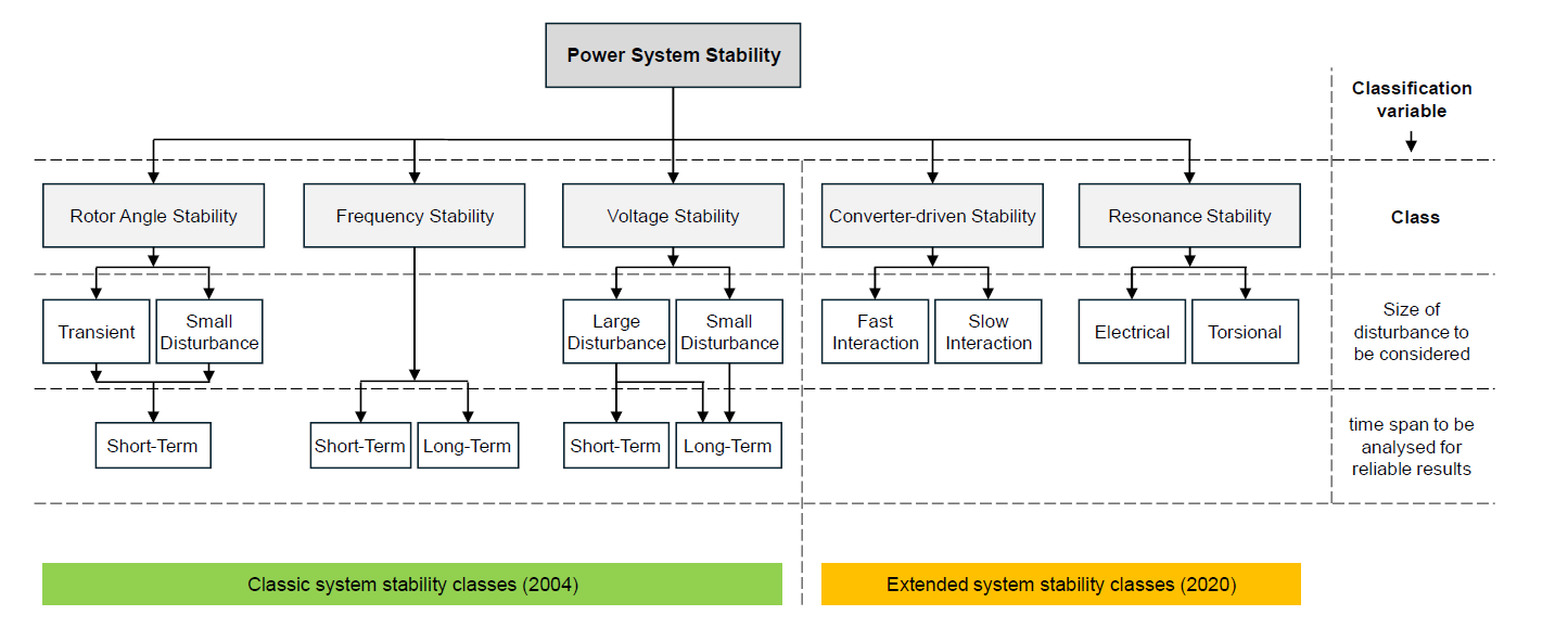
Figure 1 – Classic and extended power system stability classes according [4] and [5]
| Rotor Angle Stability | Frequency Stability | Voltage Stability | |
|---|---|---|---|
| Main system variables | Electrical and mechanical torque Te and Tm represented as power output Pel and rotor angle δ of a (group of) generator(s), bus voltages and angles Vm at power frequency | Global frequency f and system imbalance in active power ΔPsys = Pgen - Pload at power frequency | System bus voltages Vm, reactive power demand Qsys and imbalance in active power generation and load ΔPsys at power frequency |
| Size of disturbance | Small: local mode and inter-area mode oscillations (small-signal models) Large: Severe contingencies (e.g. short circuits): non-linear machine dynamics to be considered, also termed “Transient Stability”. | Small-signal models are of limited use for frequency stability analyses due to various nonlinear characteristics involved. Large signal models should be utilised. | Small: voltage stability under incremental load changes (small-signal models) Large: systems’ ability to recover after severe system faults or loss of generation (various nonlinearities). |
| Timespan | Small disturbance: 10 to 20 seconds Large disturbances: 3 to 5 and up to 20 seconds | Short-term (load shedding, nonlinear controllers): few seconds. Long-term (power plants): tens of seconds up to several minutes. | Short-term (dynamic load behaviour): several seconds Long-term (tap changers, thermostatic loads, generator and HVDC controls): several minutes |
| Analysis framework | Main system variables Pel, δ, f, ΔPsys, Vm, and Qsys are RMS values for power frequency Minimum timespan of a few seconds: phasor modelling according to power frequency | ||
3.1.2. Extended stability classes [5,6]
Hatziargyriou et al. observe that “high-frequency dynamics and phenomena, such as the dynamics associated with the switching of power-electronic converters, are represented only by either steady-state models or simplified dynamic models, meaning that fast phenomena, like switching, cannot be completely captured” and extend the theoretical definition of stability to hybrid systems as indicated in [4]. The system stability classes are extended by two classes termed “converter-driven stability” and “Resonance Stability” as shown on the right side of Figure 1. The basic structure and system stability classes of [4] are retained and the classification variables are kept unchanged.
Manifold references and real-life cases are presented for each classic stability category. Regarding rotor angle stability, light is shed onto synchronisation problems especially of GFL converters. It is noted that there is no general answer to the question of whether the integration of converters eases or exacerbates problems related to inertia and rotor angle stability, since the answer depends on the grid strength and layout as well as the converter control (during and after the fault) and position and the location of the disturbance. These statements are not new and are also valid for conventional synchronous generators. Although GFM converters are mentioned in introductory Section 2.2 of [5], they are not considered in the extended system stability classes, and it is stated that converter interfaced generation does not inherently provide inertial response. This is misleading since current GFM implementations are doing exactly that while effectively providing a voltage source behaviour in the frequency range of interest.
The new system stability class “Resonance Stability” contains interaction phenomena of different subsynchronous frequencies, which all have in common that rotating machines / generators are participating on the mode of instability. The category is further divided into torsional and electrical resonances. The term “torsional resonances” mainly refers to interactions between rotating mechanical units and an electrical network with series compensation or converter-based equipment, such as HVDC, STATCOMs or static var compensators (SVC). On the other side, ‘electrical resonances’ will describe interaction phenomena between purely electrical elements even if they are part of a larger mechanical unit, such as the induction generator effect (IGE) and SSCI.
The term “Resonance Stability” itself is misleading. It is clear, that for the effects involving a series compensated line, the resonance between the capacitance and another inductive element is the starting point for any stability investigation, but a resonance alone does not mean a stability problem as detailed in Sections A.2 and A.3 of this paper. If a resonance of a system can be measured (usually by the ratio of current and voltage), the system is obviously stable, rendering the term “resonance stability” ambiguous. The original approach of identifying the main system variables participating in the mode of instability and integrating the phenomenon in one of the existing or a new stability class is disregarded.
The new system stability class “Converter-driven Stability” includes multi-time scale control characteristics of the converters leading to the coupling interaction of electromechanical and electromagnetic dynamics between the converters and the conventional network, resulting in possible oscillations in a wide frequency range. Loosely based on the frequency range, converter-driven stability is further divided into “slow interaction” and “fast interaction”. For the former, a lower characteristic frequency (typically less than 10 Hz) will be evident, while the latter should show a higher characteristic frequency (typically from tens to hundreds of Hz, even up to the kHz level) and can be in line with the term “Harmonic Stability”. Nevertheless, the definition of a common reference frame for frequency component observations is missing. In the detailed descriptions of fast interactions, many real-life power quality issues are referenced, but no attention is paid to whether these reports are essentially power quality or stability issues. As detailed in Section A.3, there is a fundamental difference between observed resonances, harmonics and stability issues. From measured observation of voltage and current harmonics or resonances, no distinct conclusion about the system stability properties can be drawn. Equally, the details and examples presented in the description of “slow interactions” are mostly synchronisation problems of converter PLLs with various interaction frequencies and no effort is made to explicitly examine these interaction phenomena, identifying their mechanisms and the main system variables participating in the mode of instability and deriving a new power system stability class. Finally, “Converter-driven Stability“ is the only term referring to a type of asset rather than an interaction phenomenon or system variable.
Table 2 summarises the information presented in [5] regarding the classification variables forming the extended stability classes.
| Resonance stability | Converter-driven stability | |
| Main system variables | Physical quantities are not addressed. A physically based description of torsional resonance is given as a “significant energy exchange between the grid and a turbine-generator at one or more of the natural sub-synchronous torsional modes of oscillation of the combined turbine-generator mechanical shaft”. | Physical quantities are not addressed. Instead, many case studies and real-life events with high frequency interactions leading to power quality issues are presented as well as synchronisation issues around power frequency, supersynchronous oscillations due to unstable GFL control loops and virtual rotor angle loss mechanisms due to the exceeding of line power transfer limits. |
| Size of disturbance | Not mentioned, but most likely small disturbances because of multiple recommendations to use small-signal models (phasor-based) assessing resonances and the real parts of the complex impedances. | |
| Timespan | No details given | |
| Analysis framework | No clear recommendation can be given in the absence of a definition of main system variables, frequency ranges, time spans and disturbance sizes. | |
As the information in Table 2 indicates, the considerations for classification, which were established in [4] and successfully applied throughout more than one decade, have not been applied as rationales for the creation of the extended system stability classes. Consequently, the new stability classes “Resonance Stability” and “Converter-driven Stability” are highly ambiguous and do not contribute to a common understanding of the phenomena in industry and academia and more importantly, they do not provide a solid basis for model simplification and stability phenomena reproduction. A similar conclusion has been drawn in [7].
3.2. Motivation for redefining classes of power system stability phenomena
As indicated in Section 2.3, the power system stability classification in [4] assumes an undistorted signal around power frequency without phenomena at other frequencies. The existing definitions do not consider differences in terms of signal analysis between a single-frequency and a multi-frequency signal and therefore fail to appropriately include these types of phenomena. However, the properties of multi-frequency signals can be well integrated based on fundamental relationships as described by the way of example in Section A.5 for subsynchronous and power-frequency oscillations. A suitable extension of the classic system stability classes in [4] must include all relevant frequency components of phase signals as follows:
- DC: future power grids will contain substantial power generation and transmission at DC voltage, from photovoltaic and wind power connections to Multi-Terminal and Multi-Vendor (MTMV) HVDC grids. Power frequencies (i.e. 50 and 60 Hz) must be complemented with DC.
- Subsynchronous frequencies: The two most important signal forms are oscillations with a single spectral line in the subsynchronous frequency range and amplitude modulation of the power-frequency component (50/60 Hz) with one of the two spectral lines in the subsynchronous frequency range (cf. Section A.5)
- At and close to power frequency: All classic stability phenomena including local and inter-area mode oscillations in the form of frequency and amplitude modulations with spectral lines in close vicinity to power frequency.
- Supersynchronous frequencies: Spectral lines in the frequency range between power frequency and twice the power frequency may emerge from interactions between control loops and the grid (e.g. current controller in stationary reference frame) or due to frequency coupling in combination with subsynchronous phenomena [8].
- Harmonic frequencies: Frequencies ranging from twice the power frequency up to 2.5 kHz including interharmonic components according to international standards. It must be noted that this threshold has no technical/physical rationale and could in principle be chosen arbitrarily. The authors do not see any reason to readjust this value.
- Supraharmonic frequencies: All frequencies above 2.5 kHz, mostly dominated by the frequency-dependent influence of passive equipment, switching actions and control delays.
While stability phenomena at and close to power frequency can be adequately analysed in the RMS reference frame using phasor-based models (see Section A.5), phenomena at sub-/supersynchronous frequencies can be efficiently captured with EMT simulations. In conventional RMS simulations at power frequency, the system impedance matrix is assumed to be constant, and likewise for frequency deviations. The error involved in using the nominal power-frequency RMS reference frame increases with the distances of frequency components to power frequency and rises sharply as soon as the system impedance matrix deviates strongly from the nominal frequency system impedance matrix as in the case of resonances, which applies in particular to eigenmodes of torsional shafts.
The main system variables involved in the modes of instability are voltages and currents at various frequencies. These basic variables can lead to oscillating powers and torques when considering mechanical equipment but have little physical relevance if no rotating machines are involved. The classification variable “main system parameter involved in the instability mode” does not help to distinguish between the classes if interactions at sub- or supersynchronous frequencies cannot be clearly linked to a few system states or electrical quantities. For this reason, the classification variable “main system variables involved in the modes of instability” is not applicable to frequency ranges other than power frequency. The precise differentiation of the main system variables involved in high frequency interactions could be a subject for future research if deemed necessary.
3.3. Suitable classes of power system stability phenomena
Considering the aspects in Section 3.2, the frequency components must be introduced as a classification variable for all three classic stability classes associated with the power-frequency range.
The relevant frequency range of normal system operation (disconnection of generation not expected) and frequency related system ancillary services of consumers and generators in international grid codes can be conservatively summarised as power frequency ± 2.5 Hz. This range already covers typical local and inter-area mode power oscillations with spectral lines of the phase signal DFT at power frequency ± (0.1 to 2.5) Hz as explained in Section A.5. It also includes eigenmodes of assets in the range of power frequency ± 2.5 Hz, e.g. torsional eigenmodes of wind turbine drivetrains, which are typically in the range of power frequency ± (1 to 2.5) Hz [12, 13, 14]. In this class, phasor models for power frequency are the modelling assumption of choice, as all relevant dynamics can be captured, and the complex impedances of the system can be assumed constant in this frequency range.
Stability phenomena involving torsional modes of generator shafts of conventional and recent hydrogen gas power plants are typically observable in the frequency range of power frequency ± (3.5 to 40) Hz (cf. Section A.5). Eigenmodes of generator shafts can be modelled as resonances in the system impedance matrix, which let the error involved in using nominal power-frequency system impedances rise sharply as soon as frequency components get close to eigenmode frequencies. Considering both constraints, the boundary between the power-frequency range and the sub-/supersynchronous frequency range must be within 2.5 to 3.5 Hz. Pragmatically, it is best drawn symmetrically around power frequency with a spacing of 3 Hz. The derivation of physical rationales for an exact threshold might be a topic for a multi-stakeholder taskforce. While [15] presents similar ideas but does not draw clear boundaries between classes nor considers adjustments of the classification variables to form unambiguous classes, [7] recommends a frequency-dependent classification, leaving a clear boundary value to be defined. Figure 2 illustrates the proposed classification.
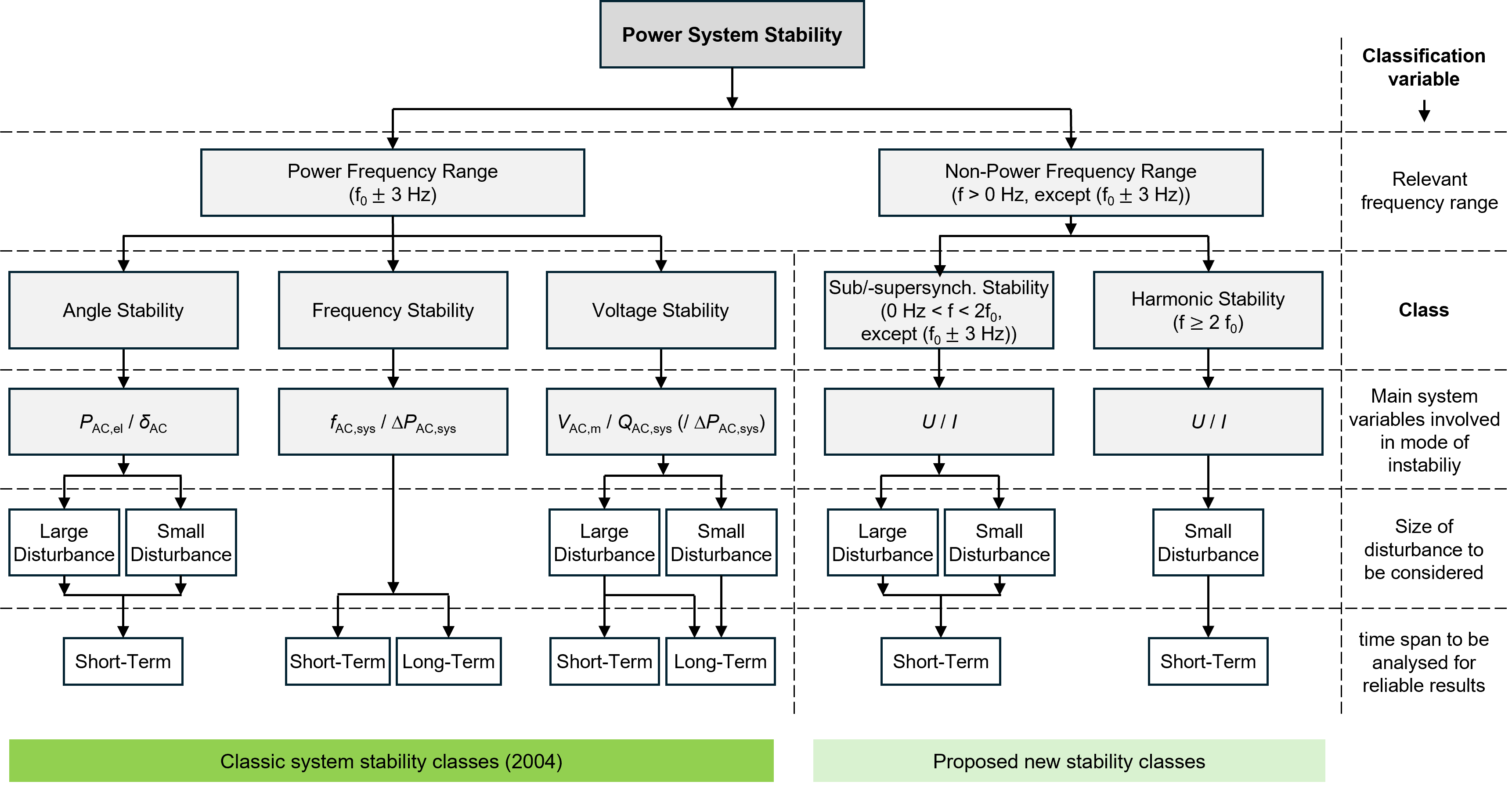
Figure 2 – Proposed power system stability classes
3.3.1. Class "angle stability"
The category “Rotor Angle Stability” should be generalised to “Angle stability” adhering to the original definition by Kundur in [9]. This category includes virtual synchronous machine concepts of GFM converters as well as other synchronisation concepts of GFL and GFM converters acting at power frequency. While “Angle stability” is associated with power frequency, stability phenomena observed in GFL PEC include a wider frequency range around power frequency. The considerations in Section VD in [16] and the detailed analysis of the PLL and current controller mechanisms leading to sub-/supersynchronous instability in [8, 17] reveal, that depending on the implementation of the current controller (e.g. reference frame: stationary or rotating) and the parameterisation of the PLL, either the frequency spectrum of the current may contain symmetrical sub- and supersynchronous spectral lines or a single-sided sub-/supersynchronous spectral line may be observable. The latter may result from the resonance of a current controller in stationary reference frame with the grid in contrast to an implementation in the rotating reference frame. Symmetrical spectral lines in currents may lead to spectral lines in voltages with different magnitudes related to the frequency dependent grid impedance and its resonances. In conclusion, the synchronisation mechanism of GFL PEC involves multiple frequencies besides power frequency and cannot be classified under “Angle Stability” but rather under “Sub-/Supersynchronous Stability”.
In view of the results of system stability studies by the German TSOs [10, 11], it should be emphasised that voltage magnitudes and angles between (groups of) generators are taken into account when investigating angle stability with large disturbances (also referred to as “Transient Stability”). This applies in particular to a small number of synchronous machines that are connected via long lines in a highly loaded grid. In this case, an angular instability of distant (groups of) generators manifests as a voltage instability in the electrical centre of the corridor. A separation between “Angle stability” and “Voltage stability” can only be achieved by defining relevant nodes, such as generator nodes at the ends of the corridor for “Angle Stability” and customer nodes along the corridor for “Voltage Stability” [4].
3.3.2. Class "sub-/supersynchronous stability"
Power system stability phenomena in the subsynchronous frequency range are associated with at least one spectral line in the subsynchronous frequency range including amplitude modulation at power frequency (cf. Section A.5). An overview of effects in the subsynchronous range such as the subsynchronous resonance (SSR) condition itself, subsynchronous torsional interaction (SSTI), induction generator effect (IGE) and numerous device dependent subsynchronous oscillations (DD-SSO) is provided in [18]. If a PEC is actively participating in an undesired interaction, this type of interaction is sometimes referred to as subsynchronous control interaction (SSCI). An SSCI-triggered oscillation is called SSO if there is a single spectral line below power frequency. If the frequency coupling effect is obvious and spectral lines in the subsynchronous (0 Hz < f < (f0 – 3 Hz)) and supersynchronous ((f0 + 3 Hz) < f < 2f0) frequency ranges are observable, it can be called “Sub-/Supersynchronous Oscillation” (S²SO) [7, 19, 20, 8]. Torsional modes are given relative to the machine rotor frequency (i.e., power frequency) and the frequency coupling results in two symmetrical spectral lines in the frequency dependent impedance of the machine just like the sub/-supersynchronous frequency coupling of GFL controllers implemented in the rotating reference frame. The symmetry around power frequency therefore means that S2SO can be observed between 0 Hz and twice the power frequency.
Generally, small disturbance small-signal models can be used for screening purposes and large disturbance EMT simulations must be employed for detailed analysis. For example, subsynchronous generator-shaft based interaction phenomena (SSTI) can be studied using small-signal Damping Torque models but must be validated with Transient Torque EMT analyses. Electromechanical equipment with relevant characteristics (e.g. multi-mass generator shafts, series compensated lines) and controls with bandwidths in the subsynchronous frequency range must be modelled. To capture all dynamics relevant for supersynchronous oscillations, system resonances up to twice power frequency must be modelled, including control loops with corresponding bandwidths like the PLL and current controller in case of GFL PEC. Higher-frequency dynamics as classified in “Harmonic Stability” can be neglected as they do not contribute to the sub-/supersynchronous resonance conditions. For S2SO, small-signal screening studies are well suited but validations and detailed analyses using an EMT simulation framework are indispensable.
3.3.3. Class "harmonic stability"
The category “Harmonic stability” covers harmonic and interharmonic frequencies for all frequencies above twice the power frequency. Harmonic Stability covers small-signal analyses, e.g. using the impedance-based stability criterion (IBSC) [24], as well as EMT simulations to account for non-linearities in control or protection schemes. It should be noted that large disturbances are relevant for harmonic studies only in the sense that they lead to a new steady-state operating point during the disturbance. During the large-signal transition, nonlinear dynamics come into play and small-signal models are not applicable. The prefault and during fault system topologies have fundamentally different harmonic characteristics and can be interpreted as different AC system configurations for harmonic stability studies, for which different harmonic PEC impedances most likely apply.
A clear distinction is needed between analyses of transient interactions at higher frequencies and stationary harmonics in terms of power quality (cf. Section A.4). Studies of transient interactions at higher frequencies evaluate the system’s transient response to an excitation, i.e. the reduction or amplification in amplitude of an oscillation of a signal at one spatial point of observation at multiple consecutive points in time and include information of all frequencies. Stationary harmonic studies analyse the stationary amplification or attenuation of an oscillating signal in form of the frequency-specific reduction or amplification in amplitude for a specific period in time at different spatial locations. Stationary phasor models of higher frequencies are the tool of choice for harmonic studies, while EMT simulations are inevitable for studies of transient interactions at higher frequencies.
As indicated in Section A.4, transient interactions at higher frequencies (e.g. control interactions) can lead to stationary oscillations, if damping is not provided or not effective. In this case, the transient interaction transforms into a power quality issue. Similarly, a harmonic stability problem with a continuous increase of a higher frequency signal amplitude can turn into a power quality issue, if the signal is limited by a non-linearity (e.g. saturation, rate-limiter, etc.) and would be observable as a stationary oscillation. If the harmonic voltage or current exceeds a (time-based) protection threshold and a nonlinear breaker action leads to the disconnection of converter-coupled generation, the power quality issue in turn transforms into a system stability issue. Both small-signal models for small disturbances and EMT simulations for validation are used from very short time spans like one power-frequency period to several seconds. Most electromechanical equipment can be assumed to be stationary during high-frequency dynamics and hence subsynchronous and power-frequency dynamics can be neglected. The frequency-dependent impedances of many PEC begin to represent operating point independence above 120 to 150 Hz, which is of great importance for power system studies. Transmission lines, cables, transformers, loads, FACTS, converters, etc. must be modelled in detail.
3.3.4. Considerations on the inclusion of assets based on DC technology into power system stability classes
So far, all considerations relating to the classification of interactions have focused exclusively on the AC side. This is justified by the fact that most of the HVDC systems are realised as point-to-point single vendor systems and that the interactions involving converters take place on the AC side. However, the planning paradigm for transmission systems is shifting towards multi-terminal and multi-vendor HVDC grids that are expected to facilitate the transportation of large amounts of offshore electricity to onshore and their distribution across the AC system, to increase the market coupling and to contribute to the overall system stability. It also cannot be ruled out, that in the future, these multi-terminal systems might be interconnected and coupled with consumers on the DC side, thus forming an extensive HVDC grid. This emerging situation raises the question of including the DC side in the stability classification to streamline the definition of compliance tests of new DC connections, derive modelling requirements, derisk future investments, etc.
Due to lack of reported and documented DC side interaction incidents, the DC side classification considerations here are based on a priori reasoning. If frequency and angle aspects from the AC side phenomena are ignored, “DC-side voltage stability” and “DC-side transient stability” remain. The DC stability aspects under consideration are shown in Figure 3.
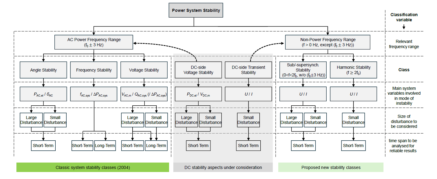
Figure 3 – Considerations on DC stability next to the proposed power system stability classes
The frequency spectra of dynamics on the DC side are transferred to the AC side by the coupling dynamics of the converter characteristics and control properties. As the literature indicates, oscillations on the DC side current with frequency ? become observable as amplitude modulations of the AC current with symmetrical spectral lines of power frequency ± ? [25, 26, 27], similar to the principles of power oscillations in Section A.5. While this can be confirmed by physical reasoning, the AC-DC-AC transfer of voltage harmonics is heavily dependent on the implemented controls and energy storages of the submodules and is still a research question to be answered.
If a new class “DC-side voltage stability” were to be introduced, its relevant frequency range might be up to 10 Hz in a stationary reference frame on the DC side since the most dominant DC voltage dynamics are typically observed in this range [28]. This frequency range might translate to power frequency ± 10 Hz on the AC side. The second DC class “DC-side transient stability” would cover the frequency range above 10 Hz on the DC side relating to the ability of the AC-DC converters to damp small oscillations within the DC system. Since converters are connected through the AC grid, the propagation of oscillations throughout the system and the interaction of multiple converters with these oscillations significantly determines the small-signal stability of the system [28]. Depending on the projection of the signal frequency spectra between the AC and the DC side, these DC-side transient stability phenomena would be classified into “Sub/-supersynchronous Stability” or “Harmonic Stability”. From the authors’ perspective, the creation of a new column next to the frequency ranges would not be useful.
4. Conclusion
The well-established classes “Rotor Angle Stability”, “Voltage Stability” and “Frequency Stability” stand in contrast to the proposed classes “Resonance Stability” and “Converter-driven Stability”. The proposed classes are highly ambiguous, do not contribute to a common understanding of the phenomena in industry and academia and more importantly, do not provide a solid basis for model simplification and the reproduction and mitigation of stability phenomena. This paper revisits the classification of power system stability phenomena and proposes an appropriate classification scheme to account for current and future converter-dominated power grids. To achieve this, the original considerations for classification are retained and two new classes “Sub-/Supersynchronous Stability” (S2SO) and “Harmonic Stability”, are established based on frequency components as additional categorisation variables to account for multi-frequency signal characteristics as well as appropriate assumptions for model simplifications.
Frequency and amplitude modulations of local and inter area oscillations observable in the RMS reference frame with oscillations of 0.1 to 2.5 Hz correspond to spectral lines in the phase signal DFT of power frequency ± (0.1 to 2.5) Hz. The relevant frequency range of normal system operation (disconnection of generation not expected) and frequency-related system ancillary services of consumers and generators in international grid codes can be conservatively summarised as power frequency ± 2.5 Hz. Stability phenomena involving torsional modes of generator shafts are typically observable in the frequency range of power frequency ± (3.5 to 40) Hz (cf. Section 4.5). Considering both constraints, the boundary between the power-frequency range and thus the classic power system stability classes, and the S2SO frequency must be within 2.5 to 3.5 Hz. Pragmatically, it is best drawn symmetrically around power frequency with a spacing of 3 Hz.
Torsional modes are given relative to the machine rotor frequency (i.e., power frequency) and the frequency coupling results in two symmetrical spectral lines in the frequency dependent impedance of the machine just like the sub/-supersynchronous frequency coupling of GFL controllers implemented in the rotating reference frame (cf. Section 3.3.2). The symmetry around power frequency therefore means that S2SO can be observed between 0 Hz and twice the power frequency. The category “Harmonic Stability” covers harmonic and interharmonic frequencies above twice the power frequency (cf. Section A.4).
A suitable classification of power system stability phenomena is proposed, which takes these characteristics into account, provides a broad overview of power system stability and enables suitable model simplifications for detailed studies. Details are explained in the relevant sections of this paper. The derivation of specific modelling requirements on the basis of the classification scheme presented is the subject of further work. While the proposed classification has been discussed with several TSOs and one manufacturer, broader discussion and consultation is suggested, e.g. through a multi-stakeholder task force.
The planning paradigm of transmission systems is shifting towards multi-terminal and multi-vendor HVDC grids that are expected to facilitate the transportation of large amounts of offshore electricity to onshore and their distribution across the AC system. If a new class “DC-side voltage stability” were to be introduced, its relevant frequency range might be up to 10 Hz in a stationary reference frame on the DC side (cf. Section 3.3.4). This frequency range might translate to power frequency ± 10 Hz on the AC side. A second DC class “DC-side transient stability” would cover the frequency range above 10 Hz on the DC side related to the ability of the AC-DC converters to damp small oscillations within the DC system [28]. Depending on the projection of the voltage frequency spectra between the AC and the DC side, these DC-side phenomena would be classified into “Sub/-supersynchronous Stability” or “Harmonic Stability”. While these basic considerations seem to hold valid, the indicated extension of the classification scheme in Section 3.3.4 is subject to further research.
In order to promote a common understanding and a common technical language, this document introduces clear and unambiguous definitions of important technical terms, including (non)-oscillatory (in)stability, damping, resonances, attenuation, amplification, passivity, harmonics, transient interactions, subsynchronous oscillations and power oscillations.

5. Annex on terminology and definitions
For clear, precise and consistent discussions, some terms and concepts need to be clearly defined and distinguished from imprecise expressions.
5.1. Power system stability
The definition of system stability by Kundur et al. [4] is valid for classic power systems governed by the dynamics of synchronous generators still present today as well as for future converter dominated power systems [6]:
“Power system stability is the ability of an electric power system, or a given initial operating condition, to regain a state of operating equilibrium after being subjected to a physical disturbance, with most system variables bounded so that practically the entire system remains intact.”
It is of great importance to note that the power system is a highly nonlinear system operating in a constantly changing environment (operating points of loads and generators, topology, etc.). When subjected to a disturbance, the stability of the system depends on internal properties such as the initial operating condition. Typically, the state trajectories of any power system are restricted to a feasible and technically permissible range. Trajectories that exit this desired region may either lead to non-linear structural changes and the formation of a new subsystem (e.g. breaker tripping), or to unsafe operation.
This nonlinearity implies that system stability cannot be evaluated for a few single possible operating points and topological structures of the system but needs to be assessed in a more comprehensive and holistic manner. As outlined in Chapter V of [4] dedicated to system theory foundations of power system stability, system stability cannot be assessed based only on normal operating conditions but must be evaluated in respect of all possible fault conditions leading to possibly more critical subsystems. If after nonlinear actions of relays and line tripping, a power system forms a subsystem with a different topology, the stability of the subsystems must also be assured in order to prevent a cascaded system failure. With the increase in power-electronic converters these subsystems are even more important, since the control and protection schemes do allow for highly nonlinear security switch off and disconnection patterns. Harmonic protection is one example that could possibly lead to the tripping of a converter, whereas it would not be any problem for conventional equipment. The increasing number of saturable controls, such as power oscillation damping (POD) or reactive power controls, or any excitations leading to current limiting of converters, are rendering large system small-signal stability analyses difficult. If nonlinearities are active and relevant, methods for nonlinear stability analyses, e.g. based on Lyapunov or hybrid systems, must be employed or the system must be split into multiple variations of the main system in accordance with the saturated signals.
5.2. (Non)-oscillatory (in)stability and damping
Different dynamic system responses can be observed based on the dominant eigenvalues involved. A stable system will eventually converge to an equilibrium point, while a globally asymptotic system does so for all initial starting points. The dynamics of a stable system can be oscillatory or non-oscillatory (asymptotic) depending on the imaginary part of the eigenvalues, while the real part of all eigenvalues must be negative for the system to be stable. An example of a dynamic system is represented by a second-order transfer function in Laplace-domain
with s, K, T, D being the complex frequency, the gain factor, the time constant and the dimensionless degree of damping of the system, respectively. The poles of G are equivalent to the zeroes of the denominator and to the eigenvalues of the transfer function in matrix form [29].
In physical systems, damping is “the loss of energy of an oscillating system by dissipation” [30]. This effectively means that damping is a characteristic feature of a transient in time domain and reflects the energy dissipated by the entire system. If the degree of damping is negative, at least one eigenvalue will have a positive real part, the energy of an oscillation at the corresponding eigenmode will increase over time and so will its magnitude. With T and K set at 1, the impact of the degree of damping D can be studied as shown in Figure 4.
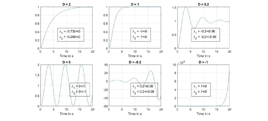
Figure 4 – Impact of the degree of damping considering a sample dynamic system represented by a second order transfer function
The following can be observed from these stylised and simplified system reactions:
- A degree of damping of greater or equal to 1 represents an energy-dissipating system with a non-oscillatory response to excitations. The real parts of the eigenvalues are negative (system is stable) and the imaginary parts are zero (non-oscillatory). The higher the degree of damping, the slower the system’s response.
- A degree of damping of zero results in a marginally stable system with an undamped response and a persistent oscillation. No energy is dissipated. The real parts of the eigenvalues are zero and the imaginary parts are nonzero indicating the angular oscillation frequency.
- A negative degree of damping characterises an unstable system which does not dissipate but supplies an oscillation with additional energy. The real parts of the eigenvalues are positive (system unstable) and the imaginary parts indicates whether the system response is oscillatory (nonzero) or non-oscillatory (zero).
The damping ratio of each system eigenvalue equals to the decay exponent of its time domain response as ??=−??{?}/|?| [31]. Damping characterises the system’s transient response to an excitation as it describes the reduction in amplitude of an oscillation of a signal at one spatial point of observation at multiple consecutive points in time. It includes information of all frequencies, and it must not be confused with stationary amplification and attenuation (negative amplification) of oscillations, which regularly occur in power systems as part of power quality. The stationary attenuation of an oscillating signal is described by the frequency-specific reduction in amplitude considering one period in time at different spatial locations. Power quality harmonic attenuation is observable in complex power systems, and also on very simple subsystems such as a voltage divider. To avoid using the expression “damping” ambiguously, it should be used to characterise the system’s transient response, while the expressions “harmonic amplification” and “harmonic attenuation” should be used for stationary power quality analyses.
Caution is advised when using the terms ”(non)-oscillatory (in)stability” since the dynamic trajectories depend on the observer’s perspective, which is the reference frame. A non-oscillatory instability in RMS values or dq0 reference frame with a steady increase in the DC component is equivalent to an oscillatory instability in stationary reference frame (abc or ??0 components) with a continuous increase in 50 Hz oscillation amplitude. In a stationary reference frame, all AC stability phenomena are oscillatory, while DC phenomena can be oscillatory or non-oscillatory.
5.3. Resonances, attenuation, amplification and passivity
To evaluate the frequency response of the transfer function G for all frequencies of interest, the stationary amplification and phase shift of G is calculated for each frequency separately, assuming an ideal sinusoidal input. The logarithmic graph of magnitude (stationary amplification) and phase shift is called a Bode plot. Following the example introduced above, Figure 5 shows the Bode plot (left) and equivalent resistances and reactances for the sample system G for each frequency (right) for degrees of damping D = 0.2 and D = -0.2.
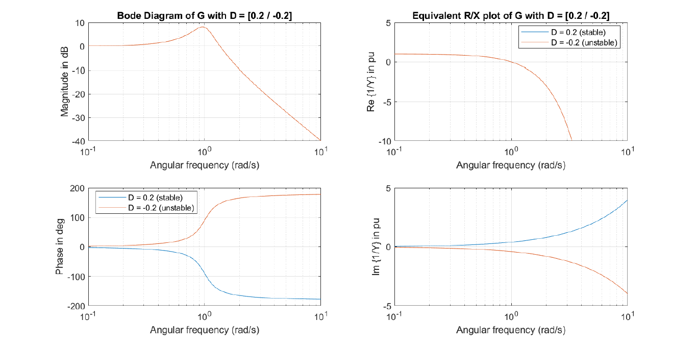
Figure 5 – Bode plot and equivalent resistances and reactances for each frequency (right) for the sample system G with degrees of damping D = 0.2 and D = -0.2
A resonance (Latin for “re-echoing”) is characterised by a strong exaggeration of the system’s magnitude amplification in comparison to an expected amplification and is a feature of the system’s stationary frequency response. The system presents a resonance frequency at 0.98 rad/s with a gain (amplification) of 8.09 dB and a -40 dB decrease per decade regardless of the degree of damping. At resonance frequency, the phase equals -84 and +84 degrees for D = 0.2 and D = -0.2, respectively. A constant ideal sinusoidal input at 0.98 rad/s would be amplified in magnitude by a factor of 8.09 dB ≈ 2.54 and phase shifted by -84 / +84 degrees. Usually, the order of the system’s transfer function is unknown, and the frequency scan results are used to parameterise electric equivalents for system studies. The equivalent electrical resistance and reactances at resonance frequency would be 0.0396 pu and 0.392 / -0.392 pu, respectively. The subsystem G is nonpassive for frequencies starting from 1 rad/s regardless of its degree of damping or stability.
It is well known that if the system “acts as a passive system, i.e., the differential input impedance has nonnegative resistance (i.e., nonnegative real part) for all frequencies, then it cannot generate instabilities” [32, 33]. Passivity and damping are obviously different concepts as passivity is determined solely by the equivalent resistance for each frequency with no time-domain characteristics, while damping is determined by the eigenvalues of the system. While a passive subsystem is always stable itself, but not necessarily when connected to another non-passive subsystem, a nonpassive subsystem is not necessarily unstable itself (cf. Figure 4 and Figure 5 for D = 0.2). Although passivity and stability are related, they cannot be directly linked.
The eigenvalue of G has an imaginary part of 0.98 rad/s corresponding to the impedance resonance peak in Figure 5. While this observation is straight-forward, the back-calculation of eigenvalues and system damping from an array of discretely sampled impedances is possible only by comparing it to known transfer functions (e.g. a second order RLC filter) or by polynomial approximation methods such as those for transmission lines in EMT simulations using the unified line model (ULM) approach [34].
To sum up, it is impossible in practice to quantify the damping inherent to a system by examining only its frequency-dependent characteristics. Equally, no detailed statements about the transient response to excitations based on the stationary frequency response are possible (only the occurrence of frequency components). Nevertheless, conclusions regarding the amplification or attenuation of stationary periodic input signals and general stability when connecting multiple subsystems can be made. The latter refers to the IBSC, which is based on the Nyquist Stability Criterion, as a screening tool for evaluating the stability of two sub-systems to be connected. Although the IBSC allows for the evaluation of discrete stationary impedances, it is essentially an evaluation of Cauchy’s integral theorem to predict unstable poles (eigenvalues) of the connected system. Finally, it is important to highlight that from measured observation of voltage and current harmonics or resonances, no distinct conclusion about the system stability properties can be drawn.
5.4. Harmonics and transient interactions
The international power quality measurement guidelines impose requirements on the accuracy of the measurement chain, the measurement time window, the Discrete Fourier Transform (DFT) parameters and the way single DFT results are aggregated to standardised bins [35, 36, 21]. Given a time-window of 10 power-frequency cycles for 50 Hz and 12 cycles for 60 Hz, each harmonic evaluation period consists of a 200 ms signal with a frequency-resolution of 5 Hz. From this, frequency bins are aggregated to “harmonics”, “intra-harmonics” and “supraharmonics”. In the case of a DFT where the frequency domain spectrum is a discretely sampled function, “both the time domain function and the frequency domain spectrum are assumed periodic” [37] and hence, power quality is a stationary phenomenon with no transient information involved. Harmonic voltages and currents can be used in various impedance-based (phasor) analyses assuming that the system is in steady state at least for a minimum duration of a few grid cycles.
Based on this information it is evident that impedance-based (phasor) models cannot be utilised to capture transient interactions of higher frequencies since a transient system is obviously not in a stationary state. Full-detail EMT simulations are necessary. It will be noted that current research in the field of dynamic phasors could play a role in future [38], but it is not clear if system studies on the basis of dynamic phasors or similar would be less burdensome than conventional EMT simulations. Furthermore, interpretation of the results is not trivial given the limitations of the methods used.
Transient interactions at higher frequencies (e.g. control interactions) can lead to stationary oscillations due to non-linearities, if damping is not provided or not effective. Such non-linearities could be saturations, rate-limiting effects or similar non-control properties. In this case, the transient interaction transforms into a power quality issue. If the harmonic voltage or current exceeds a (time-based) protection threshold (e.g. of a converter) and a nonlinear breaker action leads to the disconnection of converter-coupled generation, the power quality issue in turn transforms into a system stability issue. In fact, transient interactions at higher frequency and harmonics are two perspectives on the same problem: trying to divide interaction phenomena into different time scales to facilitate simplified modelling approaches instead of system-wide EMT simulations. If the phenomenon being investigated can be assumed to be a in a stationary state, e.g. harmonics, higher frequency phasors can be applied. EMT simulations cannot be avoided when studying transient behaviour.
5.5. Sub/-supersynchronous oscillations and power oscillations
To make an appropriate modelling assumption it is important to know which frequencies are participating in an observed oscillation or stability issue. When it comes to participating frequencies below power frequency, the literature differentiates between “subsynchronous” and “sub-/supersynchronous” oscillations, while supersynchronous is limited to twice the power frequency [7, 19, 20, 8]. Often, different reference frames are chosen, e.g. RMS of power-frequency or instantaneous values (phase signals), and hence oscillations are seen from different perspectives. In Section 3.3.2, the relevant frequency range for sub/-supersynchronous oscillations is proposed as 0 Hz < f < 2f0, except f0 ± 3 Hz in the stationary reference frame.
5.5.1. Basic considerations
A subsynchronous oscillation is characterised by the appearance of spectral lines at frequencies significantly lower than power frequency when running a DFT of the instantaneous values of a signal. This corresponds to a linear superposition of a low-frequency and a power-frequency oscillation shifting the zero-crossings of the power-frequency component of the signal. The left column of Figure 6 illustrates this phenomenon. An amplitude modulation “AM” of 50 Hz is shown in the right column corresponding to a classic power oscillation as is part of inter-area oscillations or slow control interactions [39].
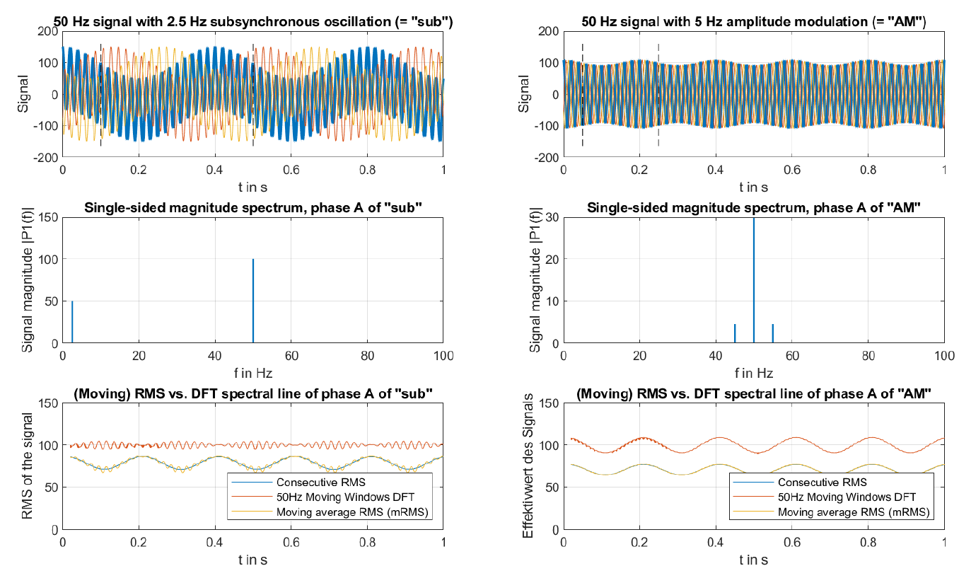
Figure 6 – Comparison of a subsynchronous oscillation (left) with an amplitude modulation of 50 Hz (right)
These two signals have been deliberately selected, as they produce the same results in a power-frequency RMS reference frame (third row, blue lines); one with a 2.5 Hz superimposed subsynchronous oscillation and one with a 5 Hz amplitude modulation (right column). The single superimposed subsynchronous frequency is visible in the magnitude spectrum at 2.5 Hz. In contrast, the two symmetrical spectral components of the amplitude modulation are close to power frequency, in this case at ??? = (?0 ± 5 ??), and do influence the magnitude only but not the zero crossings. The slower the signal frequency of the amplitude modulation, the closer the spectral components move to power frequency. Both effects contribute to the category of sub-/supersynchronous oscillations (S²SO) in Section 3.3.2.
When looking at the power-frequency RMS values often retrieved from power system measurement devices (third row, blue lines), it is not possible to distinguish between a subsynchronous oscillation and an amplitude modulation. The loss of information associated with the nonlinear RMS calculation completely obscures these phenomena. If a moving window DFT for power frequency (e.g. in accordance with IEC 61400-21-1) was used in addition to the RMS value, it would be possible to differentiate between an amplitude modulation and a subsynchronous frequency (third row, red lines).
5.5.2. Realistic phenomena
Local and inter-area mode power oscillations emerge from interactions between (groups of) synchronous generators. Figure 7 presents the scheme of a simple power oscillation test system with two synchronous generators, each being connected by one transmission line to a common load node. The length of line 13 is 5% of the length of line 23 and the total installed active power generation capacity is 1 pu. While load 1 continuously consumes an active power of 0.25 pu, the switching of the breaker of load 2 is used as excitation of the system, resulting in an additional active power demand of 0.1 pu.
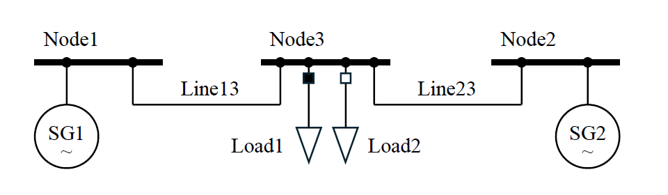
Figure 7 – Single line diagram of the sample power oscillation test system
The top row of Figure 8 shows the instantaneous voltages and currents of the synchronous generator SG1 for the first 20 seconds of this transient. While the frequency modulation of voltages and currents is depicted in the second row, the third row shows the amplitude modulation of the signals. The DFT results of the instantaneous signals are presented in the last row.
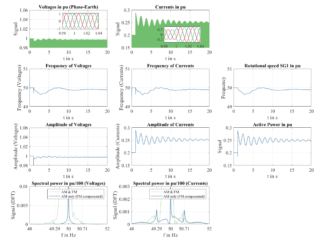
Figure 8 – Signal analysis of measured voltages and currents from the power oscillation test system
When load 2 is switched on, the balance of generation and load is disturbed, which leads to a deceleration of the rotors of both generators (cf. Figure 8, second row, right). This leads to a drop in frequency of the bus voltages and generator currents with a nadir of around 49.7 Hz as visible in Figure 8, second row left and middle. Frequency containment reserves (FCR) bring back the frequency with a steady-state deviation caused by the proportional control. The frequency plots show a slight superimposed oscillation, which arise from the interaction between the two synchronous generators without losing synchronism. Oscillating rotor angles lead to oscillating active power transfers according to the well-known relation between the sine of the angle difference and the reactance between voltage sources (Figure 8, third row, right). The almost constant amplitude of the internal voltage of the synchronous machines leads to low dynamics of the voltage amplitude at the PCC (cf. Figure 8, column 3, left). In order for the active power to oscillate, the currents must also oscillate (cf. Figure 8, third row, middle). The active power and currents continue to oscillate at power frequency, but their amplitudes vary, which corresponds to amplitude modulation. Figure 8, bottom row, depicts the typical spectrum of an amplitude modulation with two symmetrical frequency peaks around power frequency (blue graph).
Thus, local and interarea oscillations are a combination of amplitude and frequency modulation of a power-frequency carrier signal. Frequency modulation in power systems is usually associated with small modulation amplitudes of 0.1 to 2.5 Hz (often below 1 Hz) [40, 41, 42, 5]. The amplitude modulation of currents and powers leads to sideband frequencies close to power frequency, in this example to ???=50 ± 0.71?? as visible in Figure 8, fourth row, middle. Due to the proximity of the spectral lines to power frequency and the maintained synchronism of the generators, a phasor-based model can capture all relevant dynamics.
In contrast, subsynchronous oscillations as a superposition of power frequency and lower frequencies (example in Figure 6, left) cannot be analysed with phasor models but require a model that can represent more than one frequency component. Since the frequency of subsynchronous oscillation is usually unknown, comprehensive EMT models are indispensable.
Representative observed subsynchronous oscillations are presented in [19], whereas events with both sub-synchronous frequencies and amplitude modulations are listed. The authors guide through a comprehensive review of the history of the terms SSO, SSR, SSTI, SSCI and DDSSO and propose a more standardised classification based on the dominant source of the oscillation. Several publications clearly present distortions of the system by a subsynchronous oscillations shifting the zero crossings of the power-frequency component [43, 44, 45, 46]. In contrast, the events presented in [47, 8, 16, 48] feature voltages and current oscillations without a shift in the zero crossings of the power-frequency component or the introduction of half-wave asymmetry, which is mathematically possible only if by at least two complementary spectral components are involved.
Relevant torsional modes of generator shafts are typically in the frequency range of 5 to 40 Hz, which “is referenced to a ?0 rotating reference frame and indicates the modulating frequency of that ?0 carrier” [49] with ?0 being power frequency. Generator shafts of recent hydrogen gas power plants present eigenmodes even down to 3.5 Hz. Torsional modes are usually given for a rotating reference frame for power frequency and hence the frequency range of possible torsional modes corresponds to power frequency ± (3.5 - 40) Hz spectral lines in the phase signal DFT. This perspective proves what has already been clarified in [46, 9], namely that these “subsynchronous oscillations with frequencies below the synchronous frequency […] do not include electromechanical oscillations (with frequencies of 0.1 – 2.5 Hz), which are of a different nature”. Since models of the generator shaft with multiple eigenmodes and possible (non)-passivity of converters in this wide sub- and supersynchronous frequency range cannot be properly modelled in an RMS reference frame for power frequency, EMT simulations are inevitable.
References
- CIGRE, “TB 715 - The future of reliability: Definition of reliability in light of new developments in various devices and services which offer customers and system operators new levels of flexibility,” 2018.
- IEEE, “First Report of Power System Stability,” Transactions o the American nstitute o Electrical Engineers, 1937.
- IEA, “World Energy Outlook 2024,” 2024.
- P. Kundur, J. Paserba, V. Ajjarapu, G. Andersson, A. Bose, C. Canizares, N. Hatziargyriou, A. Hill, A. Stankovic, C. Taylor, T. Van Cutsem and V. Vittal, “Definition and classification of power system stability IEEE/CIGRE joint task force on stability terms and definitions,” EEE Transactions on ower Systems, 2004.
- IEEE, “PES TR-77: Stability definitions and characterization of dynamic behavior in systems with high penetration of power electronic interfaced technologies,” EEE, 2020.
- N. Hatziargyriou, J. Milanovic, C. Rahmann, V. Ajjarapu, C. Canizares, I. Erlich, D. Hill, I. Hiskens, I. Kamwa, B. Pal, P. Pourbeik, J. Sanchez-Gasca, A. Stankovic, T. Van Cutsem, V. Vittal and C. Vournas, “Definition and Classification of Power System Stability Revisited & Extended,” EEE Transactions on ower Systems, 2020.
- J. Shair, H. Li, J. Hu and X. Xie, “Power system stability issues, classifications and research prospects in the context of high-penetration of renewables and power electronics,” Renewable and Sustainable Energy Reviews, 2021.
- L. Fan, Z. Miao, S. Shah, Y. Cheng, J. Rose, S.-H. Huang, B. Pal, X. Xie, N. Modi, S. Wang and S. Zhu, “Real-World 20-Hz IBR Subsynchronous Oscillations: Signatures and Mechanism Analysis,” EEE Transactions on Energy Conversion, 2022.
- P. Kundur, Power System Stability and Control, 1994.
- The Four German TSOs, “Systemstabilitätsbericht 2023,” 2023.
- The Four German TSOs, “Netzentwicklungsplan 2037/2045 (2023),” 2023.
- J. Yang, J. Zhang and P. Wang, “Analysis of torsional vibration characteristics for wind turbine drivetrain under external excitation,” Journal o ibration and Control, Vols. 5-6, no. 31, pp. 1057-1070, 2024.
- A. Avazov, F. Colas, J. Beerten and X. Guillaud, “Damping of Torsional Vibrations in a Type-IV Wind Turbine Interfaced to a Grid-Forming Converter,” in EEE Madrid owerTech, Madrid, 2021.
- F. Fateh, W. N. Fariba and D. Gruenbacher, “Torsional Vibrations in the Drivetrain of DFIG- and PMG-Based Wind Turbines: Comparison and Mitigation,” in ASME Dynamic Systems and Control Conference, Ohio, USA, 2015.
- A. Neufeld, Zur Einordnung, Analyse und Verbesserung der harmonischen Stabilität in elektrischen Energiesystemen, 2023.
- Y. Cheng, L. . Fan, J. Rose, S.-H. Huang, J. Schmall, X. Wang, X. Xie, J. Shair, J. R. Ramamurthy, N. Modi, C. Li, C. Wang, S. Shah, B. Pal, Z. Miao, A. Isaacs, J. Mahseredjian and J. Zhou, “Real-World Subsynchronous Oscillation Events in Power Grids With High Penetrations of Inverter-Based Resources,” EEE Transactions on Power Systems, 2022.
- L. Harnefors, X. Wang, A. G. Yepes and F. Blaabjerg, “Passivity-Based Stability Assessment of Grid-Connected VSCs - An Overview,” EEE Journal o Emerging and Selected Topics in ower Electronics, 2016.
- IEEE, “READER'S GUIDE TO SUBSYNCHRONOUS RESONANCE,” EEE Transactions on ower Systems, 1992.
- J. Shair, X. Xie, L. Wang, W. Liu, J. He and H. Liu, “Overview of emerging subsynchronous oscillations in practical wind power systems,” Renewable and Sustainable Energy Reviews, 2019.
- D. Shu, X. Xie, H. Rao, X. Gao, Q. Jiang and Y. Huang, “Sub- and Super-Synchronous Interactions Between STATCOMs and Weak AC/DC Transmissions With Series Compensations,” EEE Transactions on ower Electronics, 2017.
- IEC, “TR 61000: Limits – Assessment of emission limits for the connection of distorting installations to MV, HV and EHV power systems,” 2008.
- IEEE, “519 - IEEE Recommended Practice andRequirements for Harmonic Control inElectric Power Systems,” 2014.
- EN, “50160: Voltage characteristics of electricity supplied by public electricity networks,” 2022.
- J. Sun, “Impedance-Based Stability Criterion for Grid-Connected Inverters,” EEE Transactions on ower Electronics, 2011.
- P. Li, Y. Wang, F. Li, B. Feng, Y. Liu and R. Li, “Three-Port Small-Signal Admittance Modeling and Stability Analysis of Grid-Forming MMC,” in 11th nternational Con erence on ower Electronics and ECCE Asia, 2023.
- H. Zhang, M. Mehrabankhomartash, M. Saeedifard, Y. Meng, X. Wang and X. Wang, “Stability Analysis of a Grid-Tied Interlinking Converter System With the Hybrid AC/DC Admittance Model and Determinant-Based GNC,” EEE Transactions on ower Delivery, 2020.
- L. Wang, X. Xie, J. Shair, Y. Mei and A. Lei, “Frequency-Domain Admittance Network Model (FANM) Based Oscillatory Stability Analysis of Hybrid AC-DC Systems With MMCs,” EEE Transactions on ower Systems, 2024.
- InterOPERA project, “D2.1 - Functional requirements for HVDC grid systems and subsystems,” 2024.
- R. Bishop and R. Dorf, Modern Control Systems, 12th Edition, 2013.
- M. Escudier and T. Atkins, “A Dictionary of Mechanical Engineering,” 2019.
- J. Lunze, Regelungstechnik 2: Mehrgroensysteme, Digitale Regelung, 2016.
- L. Harnefors, M. Bongiorno and S. Lundberg, “Input-Admittance Calculation and Shaping for Controlled Voltage-Source Converters,” EEE Transactions on ndustrial Electronics, 2007.
- J. C. Willems, “Dissipative dynamical systems part I: General theory,” Archive or Rational Mechanics and Analysis, 1972.
- A. Morched, B. Gustavsen and M. Tartibi, “A universal model for accurate calculation of electromagnetic transients on overhead lines and underground cables,” EEE Transactions on ower Delivery, 1999.
- IEC, “61000-4-30: Testing and measurement techniques - Power quality measurement methods”.
- IEC, “61000-4-7: Testing and measurement techniques - General guide on harmonics and interharmonics measurements and instrumentation, for power supply systems and equipment connected thereto”.
- Arrillaga, Power system harmonic analysis, 1997.
- P. de Rua, Model Transformations and Periodic Trajectory Calculations for Stability Assessments of Modular Multilevel Converter-Based Systems, 2023.
- A. Karpilow, A. Derviškadić, G. Frigo and M. Paolone, “Characterization of Real-World Power System Signals in Non-Stationary Conditions using a Dictionary Approach,” in EEE Madrid owerTech, 2021.
- ENTSO-E, “ANALYSIS OF CE INTER-AREA-OSCILLATIONS OF 19 AND 24 FEBRUARY 2011,” 2011.
- ENTSO-E, “ANALYSIS OF CE INTER-AREA-OSCILLATIONS OF 1ST DECEMBER 2016,” 2016.
- M. Klein, G. Rogers and P. Kundur, “A fundamental study of inter-area oscillations in power systems,” EEE Transactions on ower Systems, 1991.
- L. Wang, X. Xie, Q. Jiang, H. Liu, Y. Li and H. Liu, “Investigation of SSR in Practical DFIG-Based Wind Farms Connected to a Series-Compensated Power System,” EEE Transactions on ower Systems, 2014.
- X. Xie, X. Zhang, H. Liu, H. Liu, Y. Li and C. Zhang, “Characteristic Analysis of Subsynchronous Resonance in Practical Wind Farms Connected to Series-Compensated Transmissions,” EEE Transactions on Energy Conversion, 2016.
- J. Daniel, W. Wong, G. Ingeström and J. Sjöberg, “Subsynchronous Phenomena and Wind Turbine Generators,” in ES Transmission and Distribution, Orlando, Florida, USA, 2012.
- CIGRE, “TB 909 - Guidelines for Subsynchronous Oscillation Studies in Power Electronics Dominated Power Systems,” 2023.
- J. Adams, C. Carter and S.-H. (. Huang, “ERCOT Experience with Sub-Synchronous Control Interaction and Proposed Remediation,” in ES Transmission and Distribution, Orlando, Florida, USA, 2012.
- Y. Xu and Y. Cao, “Sub‐synchronous oscillation in PMSGs based wind farms caused by amplification effect of GSC controller and PLL to harmonics,” ET Renewable ower Generation, 2018.
- R. Piwko and E. Larsen, “Final Report to Research Project: HVDC System Control for Damping of Subsynchronous Oscillations,” 1982.