Applying a physics-consistent general power theory to practical electricity systems with unbalance and periodic waveform distortion – Part 2: GICs, meters and tariffs, and standards
Authors
C. T. GAUNT, H. K. CHISEPO - Dept. of Electrical Engineering, University of Cape Town, South Africa
M. MALENGRET - MLT Drives, Cape Town, South Africa

Summary
Part 1 of this comprehensive paper showed how the historical mathematical model, definition and calculations of reactive power are inconsistent with the laws of physics relevant to circuits and the concept lacks a physical interpretation. A novel general power theory (GPT) based on a measurement model that explicitly includes unbalance and distortion provides an alternative. The theory is consistent for measurement and control of power systems or an apparatus with any number of wires, unbalance, and waveform distortion. Implications were identified for volt-var control of a distributed generation inverter and for the ancillary service of reactive power compensation.
This Part 2 extends the applications to other practical problems. An analysis of voltage stability in the presence of asymmetrical distortion by geomagnetically induced currents suggests mitigation by power electronic compensation will be effective. The GPT clarifies problems with some widely used metering and tariffs in the presence of harmonic distortion and unbalance. Other implications of the theory include extending the approach to dynamic and transient applications, education, and the revision of policy and standards. However, until every application of the concept known as reactive power has been researched and replaced with physics-based alternatives, some traditional approaches will remain necessary.
The numbering and referencing in Part 2 are consistent with Part 1.
The paper is relevant to utilities engaged in electricity generation, transmission and distribution, and the regulators, manufacturers, customers, researchers, and academics.
Keywords
Apparent power – Distortion – GICs – Power factor – Metering – Power quality – Reactive power – Tariffs – Unbalance - Standards – Voltage control – Voltage stability6. GPT, GICs and voltage stability
Geomagnetically induced currents (GICs) in power systems are slowly varying currents driven by the geoelectric fields of solar storms and the voltage differences developed between grounded power network nodes. A GIC can be resolved into sinusoidal components of which the power density is mostly in the frequency range <1 to 80 mHz, so the GIC is ‘quasi-dc’ relative to the power frequency, but not constant.
A GIC flowing through a transformer’s windings and neutral-to-earth connection builds up asymmetrical part-cycle saturation of the transformer core. The transition at the magnetisation knee-point between normal and saturation flux generates odd and even harmonics of the power frequency current and gives the transformer and system a frequency dependent reactance for each harmonic in each wire.
Modelling and measurement of magnetising current and an increased reactive power in response to GICs [41] pre-dates the solar-storm-initiated Quebec blackout of 1989. It led to the formulation of “Q-loss” as an equation of GIC magnitude, p.u. voltage, and a proportionality factor k depending on the transformer core and winding type [42] [43]. This model is widely used in analysing the risk of voltage collapse [44] [45] [46].
Other studies of voltage stability and collapse associated with GICs, using commercial programs or EMT approaches, also refer to reactive power losses in transformers and a system’s increased reactive power demand, even if the parameter is measured differently [47] [48] [49].
The modelled extra reactive power increases the voltage drop in the delivery system, but symmetrical reactive power does not represent the asymmetrical transformer saturation and the system’s harmonic-distorted waveforms. Since any “reactive power values in GIC circumstances are meaningless” [50], the operational measurement and effects of the modelled symmetrical reactive power or Q-loss can only be approximations of unknown uncertainty.
This section introduces the general power theory (GPT) analysis of power flow, power loss, relative delivery efficiency, and voltage stability and compensation under conditions of waveform distortion caused by GICs. For clarity, unbalanced loads and system impedances, such as included in Section 5, are omitted here, although the GPT analysis would accommodate them.
6.1. Simple system model
The elemental model for voltage stability studies of GIC is a line and two transformers connecting a source and a load [45]. Typically, the modelling assesses waveform-symmetrical reactive power but neglects the harmonics. The procedure is to calculate the GIC flow and assign reactance to a transformer according to its per unit voltage, core type, and GIC magnitude. Then, neglecting the GIC and assuming only fundamental frequency power flow and Q-loss, the power system voltages and stability are calculated. Comparing the conventional model with one more representative of physical performance requires an EMT simulation from which the voltages, currents, and Thévenin impedances at the PoC can be extracted for a GPT-based calculation of PFSYS – the relative efficiency of delivery.
The risk of losing voltage stability arises from the current drawn through the delivery system during the period that a transformer’s instantaneous magnetising inductance ZM shown in Fig. 14 is low. The shunt inductance is non-linear, varies with time during a fundamental frequency wavelength, and can be modelled as a periodic signal with frequency components [51]. The physics-consistent GPT measurement accommodates the asymmetrical waveform distortion, frequency-dependent impedances, and unbalance caused. If compensation is applied as shown in Fig. 14, with the compensation currents defined by the GPT, the load will draw its power through the delivery system such as to minimise the losses, and voltages will improve, which reduces the risk of voltage instability.
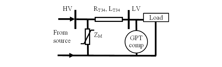
Figure 14 – GPT compensation of effects of frequency dependant magnetising inductance
A simple 4-bus system between a source and load, illustrated in Fig. 15, can be used to compare the physics-based model with the physics-incompatible model of GIC effects.
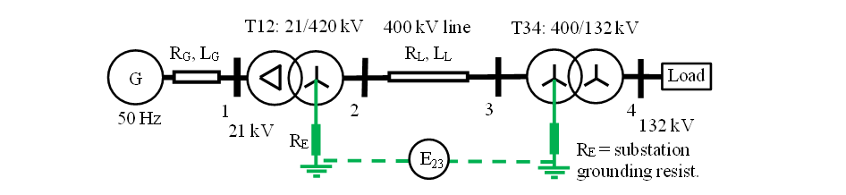
Figure 15 – 4-bus system exposed to E-field inducing GIC in ground circuit
In a similar model, the generator was modelled as a synchronous machine with internal impedance and excitation control [52]. It was shown that GPT-based compensation at Bus 4 improved the delivery efficiency and terminal voltages.
This different example examines instead the system performance without changing the generator excitation or the transformer tap ratios. The generator is modelled by an ideal voltage without impedance; in effect a power source of fixed voltage at Bus 1. The source transformer is modelled at its nominal ratio, and the load transformer at a tap-setting that delivers 1 p.u. voltage to the load at Bus 4 before the GIC is introduced.
Although most EMT programs can simulate the system behaviour with asymmetrical transformer core saturation and harmonics generated by the non-linearity of the core’s magnetisation, the saturation models of even 1-phase units differ slightly according to the software, such as between PSCAD and Matlab [53]. For simplicity in this example, the transformers are modelled as banks of single-phase units because their equivalent circuit models do not need the magnetic coupling detail of 3-phase units, which is not available in many simulators.
Values of R and X for the 3-phase banks of 1-phase 400 kV transformers are based on parameters compiled from multiple sources. The frequency-dependent transformer reactances were derived from the instantaneous inductance in Simulink as a function of the transformer flux and magnetising current. This gives a periodic signal of inductance that can be resolved by Fourier decomposition [52]. The line parameters are typical of 400 kV lines in South Africa. Table IX records the key parameters of the model.
| T12 – 3x333 MVA, 21/420 kV, nominal tap, Z=14.5 % |
| T34 – 3x167 MVA, 400/132 kV, Z=11.0 %, tap -12.5% |
| Line 23 – 250 km, R=0.0276 Ω/km; X=0.340 Ω/km at 50 Hz, neglect Y. E23=1500 Vdc |
| Load – 260 MW at 1.0 p.u. voltage, R/Z=0.96, modelled by constant Z |
| RE – substation grounding resistance 1 Ω |
For the same line type with the same conductor, line loss increases with the line length and load, but the magnitude of the GIC in long lines is not much affected by the length. The geoelectric driving voltage increases with length by the same ratio as the line resistance (which dominates the resistance of the GIC circuit), so the GIC in long lines is determined largely by the E-field. The E-field for this example is 6 V/km, which is higher than expected for an extreme event in mid-latitude regions and would represent a strong but not extreme geomagnetic disturbance in auroral regions.
6.2. Simulation
The simulation starts as a feeder operating normally, without GIC. After 10 s, the geoelectric voltage is switched on as a step-change of dc, though in a real case the GIC changes over several seconds according to the changing magnitude and direction of the E-field induced by the geomagnetic disturbance [54]. The dc representing the GIC flows through the circuit inductance, and the saturation of the transformer core increases slowly. A system settling time of about 30 s is allowed, without the generator excitation or transformer on-line tap changers compensating for voltage reduction. When the system reaches almost steady state, the voltages and currents are extracted for the GPT calculation. The transformer shunt impedance components for the level of transformer saturation are used to calculate (by network reduction) the Thévenin equivalent impedances of the feeder as seen from Bus 4. Then the GPT-based shunt compensation is introduced at Bus 4. In practice, the compensation would operate continuously with sampling of the equivalent source impedances, but the two-step approach separates the system response to the effects of the GIC from the response to compensation.
The model was implemented in MATLAB/Simulink coupled to an OPAL-RT simulator limited to a step size of 20 µs. With the accelerator turned on, an offline (without OPAL-RT) 60-sec simulation with 2 µs time step takes approximately 58 minutes.
The EMT simulation of the asymmetrical effects of GICs (represented by a constant dc current) can be compared with simulation of the Q-loss approach in this simple feeder. Q-loss is represented by inserting a shunt reactance to draw extra Q at Bus 3. The Simulink block to calculate and graph reactive power Q is accurate only without unbalance and harmonic distortion, so it cannot be used. The equivalent shunt reactance must be calculated using (a) the Q-loss based on the conventional equation and the voltage at Bus 3, (b) the change in Q at Bus 3 measured by the apparatus case of the GPT from the CRMS voltages and currents at 9.9 s and 39.9 s, and (c) using the total non-active power N=√(Q2+D2) in place of Q alone at 39.9 s.
6.3. Results
Fig. 16 shows the magnetising current in T12. Four parts of the 10-part linearised saturation model of the Matlab transformer are evident in the lower boundary of the magnetising current envelope. The two insets show the change from the magnetisation current waveform without GIC to the asymmetrical waveform 30 s later, when the response to the GIC in T12 is mostly completed. The comparable response time of the smaller transformer T34 is about 5 s.
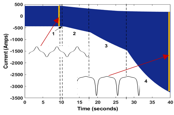
Figure 16 – Magnetising current response of T12 to GIC {t=10-40s}
Fig. 17 shows the whole current I_R in wire 1 at the PoC of the load just before compensation is implemented, and the current components h1 to h5 in all four wires resolved by Fourier decomposition. (THDi=5.5%; a gain of x12.5 is applied to the small harmonic waveforms h2 to h5.) The small difference between the fundamental frequency sinusoid in wire 1 and the actual distorted current is barely evident in the top panel. As expected, the equal triplen harmonic currents do not form a balanced 3-phase supply and, instead, sum in the neutral. The decomposition returns the angles of the components referenced to wire 1, as well as their magnitudes, but the CRMS angles will be referenced to the wire 1 voltage for the GPT input.
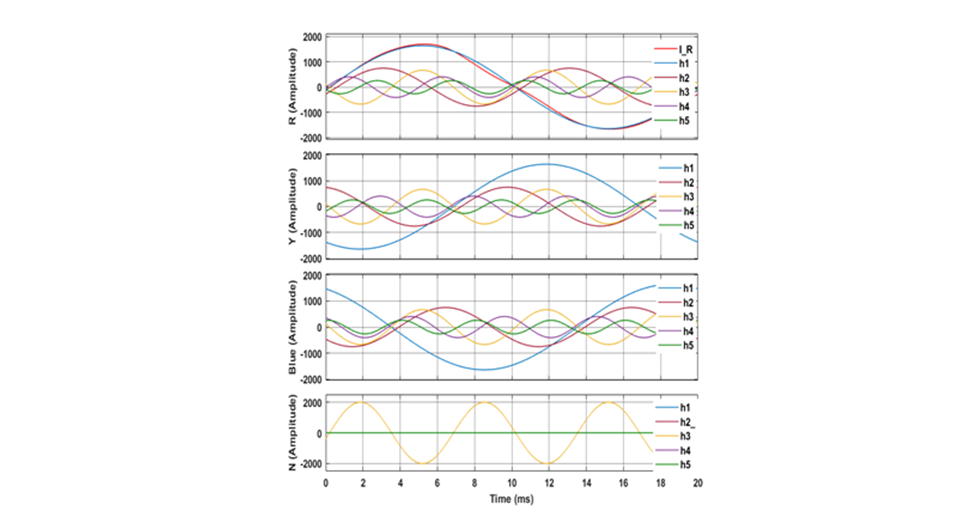
Figure 17 – Current components in GIC-saturated T34, resolved at Bus 4 at 40 s; h2 to h5 x12.5
The GIC induced in the line and transformers by an E-field of 6 V/km is approximately 126 A, represented in this model by a constant dc. The decrease of busbar voltages caused by the GIC is shown in Fig. 18. Consistent with the delayed rise of the GIC and the increase of the transformer magnetising current, the voltages take several seconds to fall. The voltage at Bus 4 decreases from 0.99 to 0.97 p.u. This decrease is just large enough that changing the transformer tap from -12.5% to -15% (usually the last tap) is insufficient to restore the Bus 4 voltage and the load at the PoC to their starting values. If the practical performance of the load with the change in terminal voltage corresponds to a constant current or constant power characteristic, the GIC would initiate a voltage collapse.
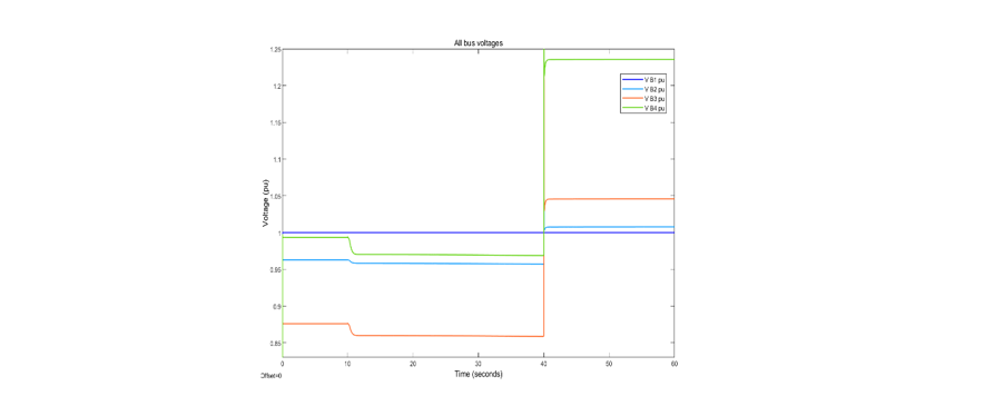
Figure 18 – Profile of bus voltage responses to GIC at t=10 s, and to the GPT based compensation at t=40 s
If the load or GIC were smaller (such as induced by an E-field of only 2 V/km), or the tap changer not as close to its limits before the GIC, the tap-changer could maintain the original voltage without reaching its limit. This explains the recommendation to reduce loading on long lines when significant GICs are anticipated [55].
The GPT-based compensation introduced at 40 s increases the voltages at Buses 2, 3 and 4, and tapping transformer T34 would return the Bus 4 voltage to its set level. (The spike when compensation is implemented is an artifact of the simulation).
Table X presents some results at Bus 4 for the normal condition, post-GIC (no compensation), and post-GIC with GPT-controlled compensation, all on fixed tap.
| Exp. | P B4 MW | VB4 pu | THDv | THDi | GPT PFSYS |
|---|---|---|---|---|---|
Normal (no GIC) | 260.06 | 0.993 | 0.187 | 0.429 | 0.8430 |
Post-GIC | 247.87 | 0.969 | 5.604 | 5.478 | 0.8401 |
Post-GIC+ GPT comp | 350.17 | 1.236 | 8.12 | 7.94 | 0.986 |
The GIC reduces the voltage and power delivered to the load, increases the harmonic distortion (THDv and THDi), and slightly reduces the system power factor. The shunt compensator then increases the voltage to 1.24 p.u., delivering more than 350 MW to the load. THDi increases because the higher voltage at Bus 3 increases the magnetizing current in the transformer, and the THDv increases as a result. The tap-changer can reduce the Bus 4 voltage to an acceptable level, which will also reduce the power delivered.
The GPT compensation of a non-linear load supplied from a linear delivery system (discussed in section 4.1) reduces the delivery loss by eliminating the harmonic power exported by the load into the feeder. Differently, in this GIC example, the GPT-based shunt compensator at Bus 4 compensates for the v-i displacement in the load, and reduces the risk of voltage collapse, but does not eliminate the distortion introduced by the GIC because minimising the delivery loss requires optimal use of all parallel lines of the superposition circuits to deliver power. Elimination of the distortion would require shunt-series compensation at Bus 4.
The GPT and the simulation clarify the role of harmonic distortion in reducing the efficiency of power delivery. They lead to the question: is the reactive power model significantly different? Given that the reactance is waveform-symmetrical, the question becomes one of how well the estimate of the magnitude of the fundamental-frequency reactance emulates the effect of the asymmetrical distortion on the voltage.
In approach (a), the magnitude of the extra Q-loss caused by the GIC is determined using the conventional equation in which k=1.18 for single phase transformers, based on tests and simulation [43]. Approaches (b) and (c) derive the change in the values of reactive power Q and nonactive power N from the full EMT simulation and the GPT apparatus case.
Table XI summarises the results of the analysis. The conventional equation exaggerates the effect of the GIC on reducing the terminal voltage.
| Approach | Add. Q-loss [Mvar] | Add’l XM [Ω] | P B4 [MW] | V B4 [p.u.] |
|---|---|---|---|---|
| Full GIC simulation | na | na | 247.84 | 0.969 |
a) Conv. Q-loss =k.V.GIC | 45.71 | 2760.41 | 242.47 | 0.955 |
b) With GPT APP: Q | 22.34 | 5860.68 | 254.58 | 0.977 |
c) GPT APP: Nonactive | 36.35 | 3524.74 | 246.14 | 0.967 |
6.4. Discussion of the GIC analysis
This example illustrates how the voltage at the receiving end of a power system is reduced by the flow of GICs. Tap changing of T34 to -12.5% (or even -15%) would not support the rated voltage and power at the PoC, which leads to progressive failure. The problem is not new. The conventional reactive-power-loss approach overestimates the voltage drop towards the limits of stability, compared with a physics-based model of system performance in the presence of harmonics. Error in the estimate of the core-type constant, k, might arise from the ambiguity in measuring reactive power loss at only the fundamental frequency, termed “effective reactive power” [56] after filtering out the distortion. The equivalent reactance that gives the closest ‘fundamental frequency’ result to a physical simulation would be based on the nonactive power (not simply the reactive power Q) of the transformer as an apparatus. The discrepancy does not appear to have been identified previously. The conventional model might be improved by revised values of k based on further research. Power electronics offers a possibility of mitigation in systems where voltage stability is a concern.
This simple example is an incomplete model. A real power system source has impedance, the lines have shunt capacitance that affects the Thévenin impedances and harmonic power dissipation, most transformers are 3-phase units with magnetic inter-phase coupling, most systems comprise many lines differently aligned with the E-field, and generator excitation and transformer tap changers respond to changing voltage. Further, GIC flow varies quite slowly, and large transformers have long saturation time constants, so the Thévenin equivalent impedances (inductances) keep changing during a geomagnetic disturbance. During periods of relatively rapid E-field change, effective compensation will require suitable approaches to measuring the system impedance parameters at approximately 10 s intervals.
In summary, the power system voltage stability is affected by (a) the stress imposed by current, voltage. and inductance harmonics, which together depend on the types of transformer construction, the distribution of transformers in the network, and the pattern of GICs during the 10-100 seconds before the worst-case stability condition, and (b) the characteristics of the generator exciters and the power electronic devices (FACTS, inverters, converters) that can change the voltage levels in the system. GPT-controlled power electronic compensation can mitigate the effects of GICs, as well as benefitting the system under normal operating conditions, but may not eliminate the distortion.
Finally, voltage stability might not be the most significant GIC-related problem for system reliability, especially as stability does not appear to have been the direct cause of outages or damage in the past. Interruptions are known to have been initiated by protection other than relays sensing instability, including tripping SVCs in Quebec in 1989, causing a blackout in Sweden in 2003, and a transformer trip on reactive-power-loss protection [57]. Although GICs have been identified as initiating transformer failure in USA (Salem, 1989), New Zealand (Halfway Bush, 2001), and South Africa (several power stations, 2003), none of the incidents were linked to voltage instability. Only models consistent with the effects of GICs on system performance can provide a reliable indication of what might happen, and how mitigation can be implemented.
7. Meters and tariffs
The validity of the GPT does not depend on implementing control for optimum loss management, though to do so may be beneficial in terms of reducing delivery losses, utility costs and carbon emissions. Fundamentally, the GPT offers consistent measurement at a connected load, source, or other network. Such measurement of losses, delivery capacity committed, and relative efficiency is the basis of electricity pricing. The financial implications of improving power quality might also affect tariffs. This section reviews some evidence of the distortion of pricing based on conventional standard-compliant metering when applied in practical systems with unbalance and distortion, and how tariffs and electricity markets are affected.
7.1. Power quality
Non-linear loads, such as fluorescent lighting, rectifiers, and variable speed drives with pulse width modulated electronic switching, draw distorted currents through even linear delivery systems and distort the voltage waveforms. Voltages distorted by GICs or over-excitation in transformers drive nonlinear currents though linear loads. Current and voltage harmonics in practical systems are directly related by the system and load impedances and cannot be separated.
Harmonic ‘pollution’ can degrade the performance of electrical equipment in various ways. Harmonics delivering energy into a resistive heating load (a sink) may be acceptable, while harmonic power that increases heating and vibration in motors is unacceptable. Generally, exported (emitted) distortion power into the delivery network, even when its source appears to be part of a load, is undesirable because the character of the nearby sinks is unknown. For this reason, nominally acceptable limits of waveform distortion are specified as part of power quality management.
Conventional power quality assessment protocols define current and voltage distortion separately. Emission limits for each harmonic order and for the total harmonic distortion of current and voltage waveforms are applied with different protocols [58] [59] [60]. The location of sources and sinks is usually based on the direction of current flow and can be supplemented by waveform measurement at all other nodes [61]. Power measurements are more sensitive indicators of sources and sinks.
Bhattarai’s Illustration 5.1 [27] of the harmonic-generating load of an arc furnace causing distortion voltage at its terminals was analysed in Section 4.1. The purpose of his example was to derive the apparent power and power factor of the load, but the real power flow is more interesting. Without compensation, the emitted harmonic power is dissipated as loss in the delivery system, which includes the impedances of all other customers – but this power cannot come from nowhere; it is derived from the power imported at fundamental frequency. The analysis in Table VI identifies the power received at fundamental frequency (PH=1=517.3 kW); the power associated with each harmonic component (total PH>1= –6 kW); and the total or nett power (PPoC = 511.3 kW). Measuring these power parameters and their direction of flow offers an alternative to the existing indices of harmonic power quality such as described in IEC TR 61000-3-6 [62] and CIGRE TB 766 [63] – even without requiring the equivalent impedances measured at the PoC.
However, for GPT-controlled compensation the equivalent impedances are required.
Shunt capacitor power factor correction of low voltage by reducing the inductance – and the voltage drop and loss associated with the non-active components of current – does not compensate for unbalance or mitigate harmonic distortion but may still be cost-effective. Passive filters for harmonic mitigation cannot adjust easily to a mix of harmonics that varies with time. Active filters controlled according to most other power theory approaches cannot compensate completely because loss reduction is not part of their derivation [64], [65].
GPT-controlled converters can respond consistently and accurately to variable distortion, v-i displacement, and unbalance. A GPT-controlled inverter has advantages for the power system. An inverter electrically close to a harmonic sink will ‘see’ low harmonic impedance and inject harmonics that will flow towards that load. Its effect will be to reduce the harmonic current drawn from a more remote source and reduce the voltage distortion on the rest of the supply system. The inverter responds also to unbalanced loads and delivery impedances.
Voltage support by energy injection from storage batteries at the grid edge could benefit from GPT control that considers the periodic waveform over a longer period such as a day or week. The power frequency is represented as a desirable high order harmonic of the longer cycle. Application of the GPT to long periods requires further research.
In summary, not all power quality mitigation approaches to distortion, unbalance and voltage control offer the same benefits.
7.2. Implications for revenue metering
The need for fair, cost-based allocation of utility prices contributed to the early development of measurable power parameters and of meters of phase displacement and unbalance [10] [66] [67]. A hundred years later, it is still important to understand where costs are incurred, whether for modern market structures that assume efficiency is achieved through cost-based competition, or for “fair” tariffs based on other factors.
Many utilities allocate costs to and levy charges for reactive power (in kvar) and reactive energy (in kvarh) measured or calculated by approved meters [68]. Strictly, these quantities are physically zero and cannot represent power or energy or the effects of phase displacement, unbalance or distortion, although meters might return a measured quantity. Other utilities charge for VA capacity or demand measured in kVA, or apply penalties based on the conventional “W/VA” power factor. Charging for these physics-inconsistent quantities of electricity or ancillary services is evident in many regulatory documents [69] [70] [71], published papers [72] [73] [74], and schedules and information sheets [75] [76] [77]. These examples of charging for defined parameters that lack physical interpretation in the power system are a tiny proportion of the worldwide use of such revenue meters and tariffs.
Most modern meters are tested by comparing the results of their calculations with specified values, rather than by the meters’ representations of a physical parameter on a physical meter test bench. Standards purporting to define or measure apparent or reactive power are based on an apparatus, not a practical supply system, so limited sets of test variables can be adopted, not always reflecting practical conditions. For example, a test might combine a sinusoidal voltage and a harmonic-distorted current, of which only the fundamental component will contribute power, and there can be no harmonic contribution to reactive power. Metering such simple arithmetic combinations of voltages and currents to give quantities of non-physical parameters is a weak basis for regulating and pricing in an economic sector as significant as electricity supply, even if the meters and tests comply with standards.
Even compliance with a metering standard does not achieve consistency of measurement between meters from different manufacturers, who do not disclose their proprietary measurement algorithms and results to the utilities, regulators or customers [15], [16]. In many countries, the regulatory jurisdiction is divided between national, state/provincial and civic governance, so resolving the technical, commercial and legal issues of metering and tariffs is complex.
Fair metering also considers the responsibility for costs incurred by distortion and unbalance in practical systems.
Bhattarai’s example exposes some typical metering issues that arise in practical systems. A non-linear load can draw power PH=1 at the fundamental frequency and export distortion as harmonic power PH>1 to be dissipated as losses. If a customer is metered and charged for the net power received at all frequencies, the quantity PPoC = PH=1 – PH>1 will be lower than the fundamental frequency power PH=1 that the system must supply. The same applies to the energy metering.
Smart meters provide such outputs of power quantities without clarifying the frequency components of the measured power [16], leading to measurements of average power exported from an installation with no generation behind the meter [17], mentioned in section 2.3. Adequate filtering in smart meters can achieve the GPT’s disaggregation of frequency components, but GPT-based meters identify the direction of power flow, and the PFSYS exposes the relative inefficiency of importing fundamental frequency power and exporting distortion.
A GPT-controlled compensator in such a system eliminates the power components of the distortion and reduces the load to PH=1. The general applicability of the GPT to systems with any number of wires, any configuration of phases, and unbalance and distortion suggests that the meter core should be more scalable and suitable for standardization than is possible with conventional meters at present. Such standardisation does not avoid choices or decisions about the practical details, such as the range of harmonics to which a meter should respond, or the uncertainty introduced by the whole measurement system.
7.3. Revisiting the 3-wire example of section 3
The example in sections 3.1 to 3.4 calculated the power parameters of the apparatus of Fig. 3 when connected to only two phases and the neutral. In a practical system, how would the meter at the PoC respond if connected instead to all three phases and the neutral, as shown in Fig. 19? A third phase wire, A, the same as the wire to terminal S, completes the 4-wire supply. According to the original example [18] [25], P=10 kW and Q=10 kvar, and this does not change.
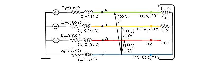
Figure 19 – Unbalanced system of Fig. 3 (with the open phase omitted and only three wires) now configured as a 4-wire system
Table XII displays some derived measurements for the 3- and 4-wire alternative supply systems. The 4-wire system can supply more power for the same loss to a load compensated to draw energy from the system with maximum efficiency. This is reflected in APSYS = 37.3 kW instead of the 35.2 kW of Table III for the 3-wire system. The relative efficiency (PFSYS = 0.272) of the practical 4-wire system is lower than the 0.289 for a 3-wire (2 phase + neutral) supply and the optimistic PFAPP = 0.324 of the original apparatus.
Parameter | CPC Apparatus | GPTAPP 3wire | GPTAPP | GPTSYS | GPTSYS | |
|---|---|---|---|---|---|---|
Power kW | 10 | 10 | 10 | 10 | 10 | |
Loss kW | - | - | - | 2.21 | 2.21 | |
Optim. loss | - | - | - | 1.85 | 1.63 | |
PF | 0.32 | 0.324 | 0.30 | 0.289 | 0.272 | |
AP kVA kW | - | 30.9 | 33.1 | 35.2 | 37.3 | |
Q kvar | 10 | 10 | 10 | Not defined | ||
DU kVA | 27.5 | 27.5 | 29.9 | |||
This example confirms the inadequacy of measuring an apparatus at the PoC, and the need to include all the wires of the delivery system.
Many meters are designed for limited wire configurations. For example, different meters are designed for a three-wire supply according to whether it is a 3-wire delta, two phases and a neutral of a three-phase system, or a centre-tapped single-phase. By contrast, the GPT can consistently measure loads connected to any 3-wire supply. Provided the voltage and current capacity of the meter are not exceeded, the same meter would measure correctly in all 3-wire systems, which promotes interoperability.
Provided a customer is billed only for power in kW and energy in kWh, no issue arises. However, when utility tariffs include traditional apparent power, reactive power, reactive energy, or power factor, the charges are unrelated to physical performance. The effects of voltage-current displacement, unbalance and distortion on supply capacity and relative delivery efficiency can be reflected only with physics-compatible models, and in this example these values differ by several per cent from conventional values.
7.4. Revenue of a generator or supplier
The DG feeder example in section 5 identified three technical aspects with economic implications: extra loss caused by VVC, payment for avoidable loss, and the ancillary service from the bulk supplier. Such aspects will become more significant as networks change from predominantly central generation to more distributed structures.
Using VVC to limit voltage rise on a feeder to enable more DG energy to be injected has little benefit for the network and customers because a large part of the extra energy injected is merely dissipated in more avoidable delivery losses. Fair energy pricing will make VVC less economic.
Secondly, the delivery efficiency from a converter interfaced DG (or battery) to an unbalanced network can be improved by injecting different currents into each wire. To be fair to the utility and customers, a DG operator should receive no revenue for avoidable loss associated with the energy output. GPT-based measurement can identify the avoidable loss, and GPT-control of the inverter can eliminate it.
At the other end of the distribution system from the DG, there are other suppliers, some of which might be expected to provide ancillary services even as their energy sales fall because of the DG’s energy input. The GPT enables the measurement of the physical parameters of the required ancillary services, such as the capacity represented by APSYS or the relative efficiency of delivery represented by PFSYS, caused by any combination of voltage-current displacement, unbalance, or waveform distortion. GPT-based metering provides a better basis for pricing than can markets or tariffs for imaginary reactive power or energy. Further, the GPT can control compensators at these intake points to minimise the effects of the non-active current components on the bulk supplier and the need for ancillary service charges.
The docket RM22-2 of the Federal Energy Regulatory Commission [78] illustrates the legal complexity of cost allocation and regulating fair payment for ancillary services. The comment by Mr Bhushan focuses on the controlled voltage parameter’s relevance, one addresses the basics of imaginary quantities of reactive power and energy [40], and 45 other responses focus entirely on pricing them.
7.5. Four-wire delta supply
In the USA, some utilities offer a 4-wire-delta supply, illustrated in Fig. 20. It can supply combinations of 3-phase 240 V loads and 1-phase 120, 208 or 240 V loads, and there is a variant with double these voltages. The transformers are three 1-phase units for a delta supply or two for an open-delta. For installations where the 3-phase load is relatively small, the centre-tapped transformer AB may have a power rating higher than the transformers AC and BC. The impedance factor R/Z (equal to conventional displacement power factor) of the various appliances can be different. Special meters (US code 85 or 95) are used [79].
Customers are often confused by how unbalanced purely resistive loads can lead to a power factor <1 and incur a tariff penalty, and utilities lack a simple way of defining the “apparent power” used in tariffs.
The effect of unbalanced resistive loading is easily illustrated in the GPT’s apparatus case. Assume the rated terminal voltages are ideal sources and three 1-phase purely resistive loads (AN=5 kW, BN=1 kW, CN=7 kW) give the wire currents directly. The power PPoC = 13 kW, and the norm of the ideal voltages from the null point is ||Vnull|| = 247.39 V. The norm of the currents, ||IS|| = 72.0 A, gives APAPP = 17.8 kVA and the apparatus impedance factor IFAPP (numerically the same as PFAPP) is 0.73, even for a purely resistive load.
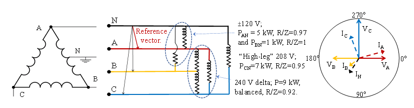
Figure 20 - Four-wire delta supply in USA: Left: Secondary winding connections. Centre: Loads, some with inductance, at the various rated voltages. Right: Vector diagram, ABC clockwise
With the ‘typical’ complex loads of Fig. 20, the power P is 22 kW, and APAPP=27.0 kVA. The GPT-based IFAPP=0.84 is higher than the 0.73 of the purely resistive loads, despite most of the appliances having inductive components.
We have not found any numerical example of this type of load with which to compare the GPT-based IFAPP and APAPP.
In practice, the customer’s loads on each phase vary. Unbalance is inherent in the 4-wire delta supply offered by utilities and is comparable with the unbalance of single-phase supplies. This raises questions about the purpose of measuring apparent power and power factor.
These examples illustrate (i) the apparatus IFAPP cannot be calculated from the R/Z of each of the wires in an unbalanced apparatus, (ii) the need for a voltage null point consistent with the laws of physics, not simply using any arbitrary reference and operational definition for measuring APAPP, and (iii) a need to consider “fit for purpose” measurement of power parameters for fair pricing.
Perhaps electricity pricing for 4-wire delta customers should comprise only simple 3-wattmeter power and energy measurements or, at least, an approach consistent with single-phase and split-phase customers?
8. Teaching, research, and policy
Reactive power is not what many engineers believe it to be, as discussed in section 3.6. Yet, despite its inconsistencies, the flawed concept is taught to engineering students as if reactive power flows in power systems and has real physical meaning. Thereafter, much academic research and thousands of papers develop more simulations using this parameter on the assumption that the conventional analytical tools prove the validity of the concept. The flawed concept is embedded further in standards, regulatory policy, and grid codes every time reactive or apparent is defined or applied. There is scope for a more evidence-based and ethical approach in teaching, research, and policy.
8.1. Teaching
How does an understanding of power theory without the concept of Q affect the teaching of electrical circuits in physics and electrical engineering?
The GPT can be introduced to electrical engineering students as a relevant application as soon as they have been taught linear algebra and the physics of circuits. The linear algebra leads directly to the conclusion that the classical definition of reactive power as orthogonal to power has no physical interpretation. Thereafter, instead of teaching P+jQ models, the focus of analysis will move naturally to physics-based approaches. For example, current flows through the network to loads (or from distributed sources) according to the voltages and impedances, with power and energy loss in the system.
Some classical examples and approaches to power flow analysis, and most electronic circuit theory, are already expressed in these terms. Where appropriate, the constant power model, as achieved by online tap changing to keep constant the voltage at the terminals of loads, will be retained by iterative adjustment of the impedance model. Students and engineers will no longer struggle with the cognitive dissonance of unrealistic interpretations of reactive power and energy.
Senior undergraduate students and postgraduate students already exposed to the concepts of the GPT have had interesting responses. Mostly, the more advanced have difficulty unlearning some of their conventional knowledge, while less senior students more quickly master the applications of the GPT to analysis and tasks like inverter control. At this stage, teaching both approaches is needed, because many analytical techniques still depend on the reactive power concept. Obviously, new teaching materials can be developed only when new approaches evolve for processes presently dependent on Q.
8.2. Research
Much engineering research is carried out to resolve differences between reality (physical behaviour) and the analysis and simulations of systems and subsystems. The gap between physical and conventionally simulated response is evident in the lack of ‘accuracy’ in compensator operation, in prices allocated to quantities that cannot reflect the cost of physical losses or capacity requirements, in system voltage calculations in the presence of GICs, and the variants of limiting voltage rise by reactive power control.
Areas where the GPT’s loss optimisation of could improve system operations (with suitable adaptations to maintain rigour and relevance) include optimum dispatch, state estimation, storage battery control, dc power flow, and design of power electronic converters.
The GPT’s direct calculation of the optimal currents needed to minimize delivery loss suggests a practical and direct application of the theory to the control of compensators and inverters. A 20 kW laboratory scale concept model has been designed [33] and has shown that the IGBT currents can be controlled in the natural (ABC) frame of reference. The control of the inverter resides on two micro-controllers, a Raspberry Pi for the GPT measurement and compensation calculations and a Texas Instrument Picolo for the switches. GPT-control has also been retrofitted to two commercial inverters, in each case adding software on the existing controllers and with a digital switch to select either control approach. Preliminary tests have been conducted [80].
Practical implementation highlights various areas where associated measurement improvements can be made. In section 3 it was mentioned that rapid changes in frequency, load or Thévenin equivalent parameters can invalidate the GPT’s control of the next cycle based on past conditions. Fast, accurate measurement of changing influencing parameters from the ‘steady-state’ are needed for appropriate responses.
Research directed to a better understanding of the physical processes and improving the models of circuits, mathematics, measurement, and control will be more efficient if fundamentally flawed theories are no longer the starting point of calculations.
The GPT’s concept model and results provoke novel thinking about power systems. For example, instantaneous power has a physical interpretation, but instantaneous reactive power does not. Also, if Q doesn’t exist in steady state, what does it represent in dynamic and transient analysis where it is widely used? Transients, such as during faults and dips, and in stability control and protection relaying, require re-thinking of the physical models of varying current, frequency, and equivalent circuit impedances.
Power electronics and the GPT together offer new control options to respond to the increasing proportions of non-synchronous sources in systems – from dc microgrids to high voltage systems. Using transient and sub-transient impedances, currents and voltages, precise power electronic control could compensate more effectively the power delivery to improve stability, especially as asymmetrical phase balance is not as constrained as in rotating machines. New approaches to solving models of the system performance, including grid-following and grid-forming converters [81], illustrate the scope for improvement. Electronic circuit theory already offers solutions for dynamic systems and transients using equivalent circuit models of current and voltage and a constant current source to replace the quadratic function of reactive power [82].
However, it must be recognised that it is not feasible to discard all analysis and control that incorporates reactive power simply because its definition and calculation is not consistent with physics. Existing empirical approximations will remain useful until every application of the concept known as reactive power has been researched and replaced with physics-based alternatives. The scope for research is enormous.
8.3. Policy, standards and regulation
The GPT without reactive power has implications for technical matters wherever reactive power is mentioned, such as for power quality assessment and limits, grid codes for the integration of distributed generation, and contractual agreements. There are economic implications for existing and proposed markets for reactive power or energy as an ancillary service, and for the many tariff and pricing structures that include charging for reactive power. These are the downstream effects of an enormous legacy of national and international standards that incorporate concepts of reactive power and energy as if they are physically measurable quantities for technical control and commercial transactions.
There should be no fundamental conflict between models of system performance and the regulatory processes of electricity supply. However, neglecting significant influencing quantities to simplify a measurement process, or promote apparent interoperability between meters, leads to empirical operational measurements and quantities that cannot be visualised in physical terms. Where the ‘evidence-based’ policy and laws used by engineers, regulators and customers are based on engineering models, standards and measurements incompatible with the physical performance of circuits, they need revision.
Change always encounter resistance, but past ‘good enough’ approaches will no longer suffice for power systems evolving technically as indicated in section 2.1 and in changing socio-economic environments. Performance improvement through physics-compatible technical innovation, and customers unhappy with being charged for a quantity of reactive energy or average power that is physically zero, will drive change. Necessary regulatory and tariff reform needs electrical engineering standards to be revised. Standards committees must choose whether to unleash or oppose technical and economic progress.
9. Definitions for power terms
The terms apparent power, reactive power and power factor each had various forms and definitions when they were introduced and used after 1890. The AIEE Annual Convention in 1920 received a joint committee report and submissions on power factor from Holtz, Brown, Silsbee, Fechheimer, Wallau, Lincoln, Fortescue, Evans, Tochio, and Pratt (all were published), but did not reach agreement. National and international controversy was still evident in 1935 when proposals were submitted to standardise terms [83].
Since then, more than one definition of P, PF, AP and Q has been included in most standards, such as in the IEC Electrotechnical Vocabulary (IEV) [12], national standards like DIN 40110 [13], and several editions of IEEE Standards for power quantities [14] and metering [84], but without uniformity. Some standards, recognising that Q alone was insufficient to describe the non-active power, added extra quadrature power components like distortion or unbalance power [13], [14], following the 1935 proposals and subsequent power theories. Arising from the various approaches and despite the adaptations, problems arise when a term has several differing definitions, when more names are assigned to terms for different circuit topologies or to reflect different conditions, or when terms are commonly applied beyond the limits of their definitions.
The GPT approach has two major advantages over conventional approaches to defining power measurements. The first is that there is no reactive or non-active power with non-power units, and all power quantities have the unit Watts. Secondly, the same definitions apply to dc microgrids, to aircraft, ship and railway systems, and to high voltage grids, irrespective of the number of wires or phases, operating frequencies, unbalance and distortion and always with the same meaning.
Most applications of power measurement are for control and metering. Most control applications require fast measurement, typically over one cycle. Most metering measures average power or total energy over many cycles and small frequency variations are tolerated. There is debate about whether metering for commercial (tariff) purposes should respond to total net power or only the fundamental frequency power delivered to customers or purchased from generators [16].
9.1. Interpretable terms
The following power terms with their interpretations apply to ac and dc systems, including 1-phase 2-wire systems, 3- and 4-wire systems with any phase relationships, and systems with more wires. In all cases where the term ‘power” is used, it means average electrical power measured in Watts for one or more whole cycles.
General terms for the RMS and complex RMS (CRMS) values of a periodic function, the norm of a value, points of connection or common coupling, a measurement reference point, an apparatus, electric power network, and average power over an integral number of cycles are presented in various mathematical or engineering texts and standards.
The terms and symbols proposed below are indicative of the physical interpretation. They might be changed in definitions to suit the nomenclature of standards.
9.1.1. Current
Resistance-weighted current of a load or source connected to a delivery system:
The resistance weighted current ||IS’|| and the active resistance-weighted current ||IA’|| are the norms of the weighted currents in a delivery system where Im,h is the harmonic component h (=0 ... H) in wire m (=1 ... M), and the dash ’ signifies weighting by a square matrix R, with M x (H+1) rows and columns, where rm,h are the Thévenin equivalent circuit resistances and the diagonal vector of the matrix is R(diag) = {(r1,0, r1,1, … r1,H), (r2,0, r2,1, ... r2,H), …, (rM,0, rM,1, … rM,H)}, and all other elements of the R square matrix are zero, giving IS’=IS R1/2 and IA’=IA R1/2 [2].
Non-active current component of a load or source connected to a delivery system:
IC is the delivery current component that contributes no power and adds to resistive loss, and it can be reduced or eliminated by compensation at the PoC of a load or source.
9.1.2. Power
In all cases, the unit of power is Watts, where 1 W = 1 J/s with the dimensions in base SI units [kg m2 s-3].
System power is associated only with the total system or its H+1 frequency components. Therefore, P1, P2, …, PH denote the fundamental and harmonic components, P0 the dc component, P>1 the total harmonic component, and P the total power.
The definitions of power at different points of a system and under various conditions are presented in Table XIII.
Term and formula | Interpretation |
|---|---|
Power at PoC | Average power over one or more whole cycles for a dc or sinusoidal frequency component, summed to give total PPoC=P0+P1+P2+…+PH. (Conventionally, I into a load at the PoC is positive, and P is positive for loads and negative for DG.) |
Delivery loss: | Minimum delivery loss uniquely associated with the load or source at the PoC, possible with optimally distributed current components IAm,h. It is the sum of the loss components IAm,h2rm,h where rm,h is the Thévenin equivalent circuit frequency-dependent resistance of the delivery wire m. {Note: The value of the minimum power loss defined as ||IA’||2 is an underestimate of the total loss associated with the power at the PoC because it omits a cross product term that depends on the magnitudes of other loads not measurable at the PoC – see section 5.1.} |
Loss without compensation | Sum of the minimum delivery loss and the avoidable delivery loss associated uniquely with the uncompensated power PPoC delivered to a load or sent out from a source. |
Thévenin power Attributable Thévenin power | Attributable power at the Thévenin equivalent point is power delivered to the PoC plus power dissipated in delivery without compensation, or for a generator the power received at the Thévenin point from an uncompensated source at the PoC |
Optimum Thévenin power | The minimum (optimum) attributable power at the Thévenin point sent out to a load, or maximum received from a generator at the PoC. |
Optimum Thévenin power for same loss | The maximum power that can be sent from the Thévenin equivalent point to a load at the PoC, or received at the Thévenin equivalent point from a source at the PoC, for the same delivery loss as incurred by the uncompensated load or source. ISO' is an optimally distributed set of resistance-weighted current components such that ||ISO'||2 = PLoss and ||VTh'|| is the set of resistance-weighted voltages at the Thévenin equivalent point from a reference null point determined in accordance with Kirchhoff’s voltage law. |
- Note 1: The power loss defined as ||IS'||2 and the avoidable loss are underestimated because they omit other loads not measurable (observable) at the PoC, and are overestimated for mixed loads and sources.
- Note 2: PMTP has the equation and interpretation of APSYS but it is a real power quantity. The origin of the term ‘apparent power’ associated with an uncompensated load at the PoC was that it represented the total source output that gave losses higher than expected from a comparable dc system [10]. The APSYS (or PMTP) is the power that could be sent out for the same loss under optimum current distribution, and is consistent with the original meaning. An alternative new term could be adopted.
9.1.3. Power Factor
Power factor of a load or source connected to a delivery system:
The power factor of a load or source at the PoC is an index of the relative efficiency (or relative effectiveness of utilization) of the delivery of power through the system, and can be calculated from:
- the losses PFSYS = √(PLoss_Min/PLoss) or
- the R-weighted currents PFSYS = ||IA'||/||IS'|| or
- the power: PFSYS = |POTP/PMTP|
All these ratios of PFSYS are equal and dimensionless.
is associated with the load/source at PoC as measured, whether any compensation is implemented or not. Unity power factor, PFSYS =1, is achieved when the currents at the PoC are compensated to ||IA'|| and incur the minimum possible line loss for the total active (or average) power transmitted from a source for the power PPoC. Unity power factor has the interpretation that delivery loss cannot be reduced further by additional or different compensation.
9.1.4. Terms for an apparatus
As described in section 3.4, power-related parameters can be defined for an apparatus connected to an ‘ideal’ zero-impedance delivery system. The parameters cannot be interpreted as power in the context of circuit theory, or as being related to power dissipated as losses, but might have other uses.
The apparatus apparent power APAPP = ||Is|| ||Vnull|| is the product of the norms of current and voltage, where voltage is defined as being measured from a null point complying with Kirchhoff’s voltage law. The VA rating of an apparatus is the product of the rated currents and voltages, balanced and undistorted. The special unit VA can be retained, but the term should not refer to power and an alternative to APAPP seems desirable.
The conventional power factor is a ratio based on an operational measurement of apparent power for single-phase or balanced loads. The early term impedance factor is more suitable, giving IFAPP = Requiv/Zequiv = PPoC/APAPP. Without unbalance or distortion, the impedance factor is equal to the conventional power factor, and IFAPP=1 when reactance X=0 and the load is resistive. Although individual ratios of R/Z for each terminal of unbalanced loads cannot be combined to derive IFAPP for a whole apparatus, the individual wire terms may be useful for describing an apparatus in a system.
9.2. Operational measurement constraints
Operational measurement details do not change the validity of the definitions, and only modify for practical purposes how some power parameters are measured or metered. There are many possible constraints, including the following.
- Averaging of power (and other measurands) over 10/12 cycles, 3 s, 10 min are defined in some standards for revenue metering. Other periods for block or sliding window metering might be appropriate for control and instrumentation.
- Integral cycle control upsets most power metering. Where applied with supply off for N out of T cycles, the fundamental period for optimum loss control would be the T power frequency cycles, or a multiple of T, and the GPT would define that as the dominant frequency, with the power frequency as a harmonic component. T is variable, which could be addressed by standardisation, adaptive measurement, or single-cycle measurement and aggregation at longer intervals.
- Some standards for revenue metering require the non-fundamental harmonic components to be filtered out of the signal, while others require harmonics to h=20 to be included in a measurement and higher order harmonics excluded. Based on Section 7.2 there appears to be a case for fundamental frequency metering of power and energy, with harmonic frequency metering for power quality tariffs.
- The accuracy and precision of metering and control depends on the type and quality of the sensors, transducers and instrument transformers delivering the voltage and current signals to the meters. For example, some components in the signal channel have decreased sensitivity with increasing frequency. More suitable sensors or frequency-weighted correction factors can be used where justified to reflect the effects of high order harmonics.
- In steady state with constant frequency, equivalent impedances, and PoC load, it is unnecessary to define a starting point on wave in a particular wire for a measurement. In practical systems, small frequency changes occur all the time. The GPT requires simultaneous sampling of the inputs, and accurate determination of the cycle or wavelength so that the Fourier decomposition extracts the harmonic components correctly. Over a small number of cycles in changing conditions, instruments measuring cycles by zero-crossing or peak values may return different quantities. The difference is not significant for meters measuring power and energy over a long duration.
- The length of a periodic signal can be selected according to the control application. If energy is stored in the converter for extraction and return of energy during the period, and there are small changes of power during adjacent cycles, adequate storage for a period of 10 power frequency cycles would allow the periodic waveform to be measured and controlled over 10-cycle periods. More energy storage capacity would be needed for a weekly cycle.
The GPT is consistent for measurement and control, but the variations above need to be reviewed, defined, or standardised according to the application. Existing definitions based on the PQS triangle for an apparatus are inconsistent, not interpretable as physical quantities, and not easily adapted for the various conditions identified above.
10. Conclusion
The GPT is based on a novel power system concept model that explicitly includes the influencing quantities omitted from the conventional measurement model of the power triangle, and consistently complies with the laws of physics of circuits. Its fundamentals are that the currents and voltages at the equivalent source must be in-phase for maximum delivery efficiency, and the currents must be inversely proportional to the line resistances. The law of conservation of energy and Kirchhoff’s current and voltage laws together establish the reference for measuring voltages at the Thévenin equivalent source. The GPT applies uniformly to systems with any number of wires, dc and ac, unbalance, and harmonic distortion, which can contribute to interoperability. It enables the measurement of power parameters attributable to a load or source connected at a PoC, and the control needed to minimise the delivery loss.
Most standards and power theories are based on the PQS power triangle of an apparatus. Real power measured at a PoC is the same for any chosen reference point for voltages, and reactive power has been usefully applied to ideal balanced and sinusoidal systems. However, reactive and apparent power measurements vary according to the voltage reference used. As a result, different equations are formulated for different combinations of phase and neutral wires. Unbalanced multi-wire systems and distorted waveforms are usually neglected in equations of apparent and reactive power, or are quantified by non-physical operational definitions.
Reactive power and energy have zero average physical value over a cycle, so they cannot represent physical quantities even in balanced power systems. In unbalanced systems, the arithmetic identity S2=P2+Q2 is always inadequate despite proposals of additional non-active power terms that similarly lack clear physical meaning in circuits.
Our research shows the power parameters of an apparatus are complemented by considering the whole power system. Several examples of system performance have been studied using the GPT’s frequency domain formulation together with time domain EMT simulations. The GPT approach suggests alternatives to conventional volt-var control of DG and reactive power as an ancillary service, and to the measurement and mitigation of the effects of GICs on voltage stability. In all the examples, the fundamentally flawed concept of reactive power leads to inappropriate engineering and commercial decisions. Conventional measurement and control can be improved using the GPT, with benefits for system operation, losses, and voltage control.
Optimum GPT-control does not require communications and central coordination but could be distributed to every PoC where it is justified, which is an advantage for the resilience of systems. More broadly, the GPT offers new insights into power quality, metering and tariffs, and standards and regulatory processes.
Other early concepts in electrical engineering and physics later turned out to lack physical validity. For example, the transmission of light and radio waves through the ether was eventually disproved – the ether concept was incorrect and unnecessary. In such cases, new models and measurement processes are adopted. Similarly, for technical and economic reasons, it appears time to adopt concepts and models more representative of power system behaviour and discard the fundamentally misconceived reactive power, despite it having become part of engineering thinking.
In discussions, we are told the power triangle and reactive power cannot be replaced because they are foundational for every electrical engineer and student. Like other significant innovations, the advantages gained by early adopters of the physics-based models of system performance will eventually outweigh the reluctance to change. Students and young researchers are best placed to learn the new theory without the confusion of the old ways. The legacy of standards, conventional meters and regulatory policies relating to reactive power will take longer to rectify, but even they will change in response to new benefits from new technologies and customer opposition to tariffs for physically zero quantities.
More research is needed to replace the accumulated analytical approaches, software, system control protocols, and policy founded on misleading power theories. Some of the concepts in the GPT might be extended to transient conditions.
Meanwhile, evolving power systems with increasing proportions of renewable energy, energy storage, and power electronic converters are changing the nature of electricity delivery. The GPT’s innovative conceptual, measurement, and control approaches can contribute widely to meeting the objectives of efficiency, reliability, stability, and fairness of delivery of energy in grids that thereby become smarter.
Acknowledgements
We are grateful to the anonymous reviewers for their valuable comments on both papers. Any errors in these papers are the responsibility of the authors.
The research has been funded in part by a grant from the Open Philanthropy Project.
References
The following references cited in Part 1 are relevant also in Part 2.
[2] M. Malengret and C. T. Gaunt, “Active currents, power factor, and apparent power for practical power delivery systems”, IEEE Access, 2020 doi: 10.1109/ACCESS.2020.3010638.
[10] F. B. Silsbee, “Power factor in polyphase systems”, Trans. AIEE, vol. 39, issue 2, p1465-1467, 1920. doi: 10.1109/T-AIEE.1920.4765336.
[12] Electropedia, IEC Electrotechnical Vocabulary, available online at http://dom2.iec.ch/iev.
[13] DIN 40110 Quantities used in alternating current theory; Part 1 (1994): Two-line circuits; Part 2 (2002): Multi-line circuits.
[14] IEEE Standard definitions for the measurement of electric power quantities under sinusoidal, nonsinusoidal, balanced, or unbalanced conditions, IEEE Standard 1459-2010.
[15] NEMA C12.24 TR-2011 “Definitions for calculations of VA, VAh, VAR, and VARh for poly-phase electricity meters” 2011, National Electrical Manufacturers Association, Rosslyn, USA.
[16] A. J. Berrisford, “Smart meters should be smarter”, IEEE Power and Energy Society General Meeting, San Diego, USA, 2012. doi: 10.1109/PESGM.2012.6345146.
[17] C. Ndungu, private communications, Sep 2020 – Nov 2021.
[18] L. S. Czarnecki and P. D. Bhattarai, “Reactive compensation of LTI loads in three-wire systems at asymmetrical voltage,” Int. School on Nonsinusoidal Currents and Compensation (ISNCC), Lagow, Poland, 2015 doi: 10.1109/ISNCC.2015.7174712.
[25] L. S. Czarnecki and P. D. Bhattarai, “Currents’ physical components (CPC) in three-phase systems with asymmetrical voltage,” Przegląd Elektrotechniczny, R. 91, Nr. 6/2015, doi: 10.15199/48.2015.06.06.
[27] P. D. Bhattarai, “Powers and compensation in three-phase systems with nonsinusoidal and asymmetrical voltages and currents.” PhD dissertation, Louisiana State University, 2016. Online
[33] P. Jankee, M. Malengret, D.T. Oyedokun, C.T. Gaunt, 2022: An inverter controlled by the General Power Theory for power quality improvement. SAUPEC, Durban, doi: 10.1109/SAUPEC55179.2022.9730729.
[40] C. T. Gaunt, “Comments in response to notice of inquiry: Reactive power capability compensation,” in Federal Energy Regulatory Commission, Docket No. RM-22-2, 17 Feb. 2022.
The following references apply only in Part 2.
[41] D.H. Boteler, R.M. Shier, T. Watanabe, and R.E. Horita, “Effects of geomagnetically induced currents in the B.C. Hydro 500 kV system,” IEEE Trans. Power Del.,, Vol. 4, No. 1, pp818-823, 1989, doi: 10.1109/61.19275.
[42] R. A. Walling and A. N. Khan “Characteristics of transformer exciting current during geomagnetic disturbances,” IEEE Trans. Power Del.,, Vol. 6, pp: 1707–1714, 1991, doi: 10.1109/61.97710.
[43] X. Dong, Y. Liu, and J. G. Kappenman, “Comparative analysis of exciting current harmonics and reactive power consumption from GIC saturated transformers,” IEEE PES Winter Meeting, pp. 318-322, 2001, doi: 10.1109/PESW.2001.917055.
[44] A. B. Birchfield, K. M. Gegner, T. Xu, K. S. Shetye, and T. J. Overbye, “Statistical considerations in the creation of realistic synthetic power grids for geomagnetic disturbance studies,” IEEE Trans. Power Syst., vol. 32, no. 2, pp. 1502–1510, 2017, doi: 10.1109/TPWRS.2016.2586460.
[45] T. J. Overbye, K. S. Shetye, Y. Z. Hughes, and J. D. Weber, “Preliminary consideration of voltage stability impacts of geomagnetically induced currents,” IEEE/PES General Meeting, 2013, doi: 10.1109/PESMG.2013.6673068.
[46] I. I. Malek, M. Z. Islam, M. Hasan, M. S. Rahman, and A.H. Chowdhury, “GIC effects on 400 kV transmission lines of Bangladesh power system,” 11th Int. Conf. Electrical and Computer Engineering, Dhaka, 2020, doi: 10.1109/ICECE51571.2020.9393114.
[47] L. Kang, B. He, P. Yang, and X. Dong, “Analysis on the impact of geomagnetic storm on reactive power and voltage in extra high voltage power grid,” Proc. E3S Web of Conferences, 2019, doi: 10.1051/e3sconf/201911802049.
[48] L. Gong, Y. Fu, M. Shahidehpour, and Z. Li, “A parallel solution for the resilient operation of power systems in geomagnetic storms,” IEEE Trans. Smart Grid, vol. 11, issue. 4, pp. 3483–3495, 2020, doi: 10.1109/TSG.2019.2962669.
[49] Z. M. Khurshid, N. F. Ab Aziz, Z. A. Rhazali, and M. Z. A. Ab Kadir, “Impact of geomagnetically induced currents on high voltage transformers in Malaysian power network and its mitigation,” IEEE Access, 2021, doi: 10.1109/ACCESS.2021.3135883.
[50] H. Kirkham and D. R. White, “Reactive power and GIC: the problems of an unrecognized operationalist measurement,” IEEE Int. Workshop on Applied Measurements for Power Systems (AMPS), Bologna, 2018, doi: 10.1109/AMPS.2018.8494870.
[51] H. K. Chisepo, C. T. Gaunt, and L. D. Borrill, “Measurement and FEM analysis of DC/GIC effects on transformer magnetization parameters,” IEEE PowerTech, Milan, 2019, doi: 10.1109/PTC.2019.8810423.
[52] H. K. Chisepo and C. T. Gaunt, “Towards asymmetrical modeling of voltage stability in the presence of GICs,” IEEE PowerAfrica, Kigali, 2022, doi: 10.1109/PowerAfrica53997.2022.9905396.
[53] P. Jankee, H. K. Chisepo, A. V. Adebayo, D. T. Oyedokun, C. T. Gaunt, “Transformer models and meters in MATLAB and PSCAD for GIC and leakage dc studies,” SAUPEC, Cape Town, 2020, doi: 10.1109/SAUPEC/RobMech/PRASA48453.2020.9041060.
[54] M. J. Heyns, C. T. Gaunt, S. I. Lotz, and P. J. Cilliers, “Data driven transfer functions and transmission network parameters for GIC modelling,” Electr. Power Syst. Res., 188 (2020), doi: 10.1016/j.epsr.2020.106546.
[55] NPCC, “Procedures for solar magnetic disturbances which affect electric power systems,” Northeast Power Coordinating Council, New York, 1989, revised 2007, online.
[56] L. Marti, J. Berge, and R. K. Varma, “Determination of Geomagnetically Induced Current Flow in a Transformer From Reactive Power Absorption,” IEEE Trans. Power Del., Vol. 28, No. 3, 2013, doi: 10.1109/TPWRD.2012.2219885.
[57] C. T. Gaunt, P. J. Cilliers, M. J. Heyns, S. I. Lotz, H. K. Chisepo, et al., “Calculations leading to voltage stability and transformer assessment in the presence of geomagnetically induced currents,” CIGRE Session, Paper C4-113, 2020.
[58] D. Fallows, S. Nuzzo, A. Costabeber, and M. Galea, “Harmonic reduction methods for electrical generation: a review,” IET Gener. Transm. Distrib., Vol. 12 Iss. 13, pp. 3107-3113, 2018, doi: 0.1049/iet-gtd.2018.0008.
[59] I. Papič, D. Matvoz, A. Špelko, W. Xu, Y. Wang, et al., “A benchmark test system to evaluate methods of harmonic contribution determination,” IEEE Trans. Power Del., Vol. 34, No. 1, 2019, doi: 10.1109/TPWRD.2018.2817542.
[60] M. Pourarab, J. Meyer, M. Halpin, Z. Iqbal, and S. Djokic, “Interpretation of harmonic contribution indices with respect to calculated emission limits,” 19th Int. Conf. on Harmonics and Quality of Power (ICHQP), Dubai, 2020, doi: 10.1109/ICHQP46026.2020.9177886.
[61] P. S. Wright and P. N. Davis, “Estimation of the location of sources and sinks of harmonic power using low voltage phasor measurements in distribution grids,” Conf. Precision Electromagnetic Measurements, Paris, 2018, doi: 10.1109/CPEM.2018.8501058.
[62] IEC TR 61000-3-6, Electromagnetic compatibility (EMC) - Part 3-6: Limits - Assessment of emission limits for the connection of distorting installations to MV, HV and EHV power systems, International Electrotechnical Commission, 2008.
[63] JWG C4/B4.38, “Network modelling for harmonic studies,” Technical Brochure TB 766, CIGRE, Paris, 2019.
[64] P. Jankee, D. T. Oyedokun, and H. K. Chisepo, “Network unbalance compensation comparison: conventional pq theory vs the general power theory,” IEEE PowerAfrica, Kigali, 2022, doi: 10.1109/PowerAfrica53997.2022.9905291.
[65] H. K. Chisepo, C.T. Gaunt, and P. Jankee, “Applying and comparing the general power theory compensation for unbalance and harmonics,” Universities Power Engineering Conf. (UPEC), paper 147, Istanbul, 2022, doi: 10.1109/UPEC55022.2022.9917879.
[66] P. M. Lincoln, “Rates and rate-making,” Trans. AIEE, vol. XXXIV, Issue: 2, 1915, doi: 10.1109/T-AIEE.1915.4765295.
[67] C. Fortecue, “The measurement of power in polyphase circuits,” 1923, Trans. AIEE, vol. XLII, pp. 358-375, 1923, doi: 10.1109/T-AIEE.1923.5060878.
[68] A.E. Emanuel (Chair, IEEE WG on nonsinusoidal situations), “A survey of North American electric utility concerns regarding nonsinusoidal waveforms,” IEEE Trans. Power Del., Vol. 11, No. 1, pp. 73-78, 1996, doi: 10.1109/61.484003.
[69] Principles for efficient and reliable reactive power supply and consumption, Federal Energy Regulatory Commission, Washington, 2005, online.
[70] Electricity pricing policy (EPP) of the South African electricity supply industry, Department of Minerals and Energy, Notice no. 1398, 19 Dec 2008, Government Gazette, Pretoria, vol. 522, no. 31741.
[71] Balancing and settlement code (BSC): Improving the allocation of reactive power flows between import and export metering systems (P266), 2011, Office of the Gas and Electricity Markets Authority, London, online.
[72] C. Tufon, A. Isemonger, B. Kirby, J. Kueck, and F. Li, “A tariff for reactive power,” IEEE/PES Power Systems Conf. and Exposition, Seattle, 2009, doi: 10.1109/PSCE.2009.4839932.
[73] D. Viera, R. A. Shayani, and M. A. G. de Oliveira, “Reactive power billing under nonsinusoidal conditions for low-voltage systems,” IEEE Trans. Instr. and Measurement, vol. 66, no. 8, pp. 2004-2011, 2017, doi: 10.1109/TIM.2017.2673058.
[74] R. Konidena, “A proposal for compensating reactive support and voltage control in MISO market,” The Electricity Journal, vol. 33, 2020, doi: 10.1016/j.tej.2020.106785.
[75] Understanding kVA and kVAr charges for major customers, Ergon Energy, online.
[76] Reactive power compensation: How to unlock new revenue opportunities for solar and storage projects, Solar Energy Industries Association, 2020, Online.
[77] Tariffs & charges booklet 2021/2022, Eskom, South Africa, 2021.
[78] Docket RM22-2 of the Federal Energy Regulatory Commission, available online.
[79] ANSI C12.1-2014 American National Standard for Electric Meters – Code for Electricity Metering
[80] P. Jankee, L. Schmidt, C.T. Gaunt, M. Malengret, K. Litsoane, R. Yorke, “Design, performance and testing of a converter under General Power Theory control,” CIGRE Southern Africa Regional Conf., 2023.
[81] M. Paolone, T. Gaunt, X. Guillaud, M. Liserre, S. Meliopoulos, et al, “Fundamentals of power systems modelling in the presence of converter-interfaced generation,” Electr. Power Syst. Res., 189 (2020), doi: 10.1016/j.epsr.2020.106811.
[82] A. Pandey, M. Jereminov, G. Hug, and L. Pileggi, “Improving power flow robustness via circuit simulation methods,” IEEE/PES General Meeting, 2017, doi: 10.1109/PESGM.2017.8273753.
[83] H. L. Curtis and F. B. Silsbee, “Definitions of power and related quantities,” Electrical Engineering, vol. 54, issue 4, pp. 394-404, 1935 doi: 10.1109/EE.1935.6539147. (Discussion in vol. 54, issue 10, doi: 10.1109/EE.1935.6540733, and vol. 55 issue 2, doi: 10.1109/EE.1936.6540586.)
[84] IEEE Master test guide for electrical measurements in power circuits, IEEE Standard 120-1989.