Circuit Breaker Recovery Voltage Pole Factor Calculation
Author
D.F. PEELO - Consultant

Summary
At current interruption circuit breakers are exposed to power frequency recovery voltages which depend on the switching duty and may exceed rated system voltages. The calculation of the recovery voltages, designated by the term pole factor and expressed in per-unit (pu), is described for fault current interruption in effectively and non-effectively earthed systems and also for inductive and capacitive load current switching. The early historical treatment of recovery voltage calculation is examined in an appendix.
Keywords
Circuit breakers – current interruption, pole factors, recovery voltage, transient recovery voltages1. Introduction
Transient recovery voltages (TRVs) following short circuit current interruption consist of two components, a power frequency component and a superimposed oscillatory component. The latter component and its calculation is discussed in an earlier CSE paper [1] and the intent of this paper is to explain the calculation of the former component, in particular its magnitude in per‑unit of rated voltage.
In 1918 C.L. Fortescue of Westinghouse published an AIEE paper on symmetrical components enabling for the first time a method for dealing with three-phase unbalanced circuits [2]. The method as described in the paper applied to n-phase systems in general and its specific application to three-phase systems later relied mainly on contributions from engineers at both Westinghouse and General Electric (GE) and this evolution is discussed in the appendix.
In the following the basic principles of using the symmetrical component method are described and then applied to the cases of fault current interruption and capacitive and inductive load current switching.
2. Symmetrical Component Method
The method enables an unbalanced three-phase network, phase sequence abc, to be represented by the sum of three sequence networks designated as follows: first a balanced three-phase positive sequence network, phase sequence abc, second a balanced negative sequence network, phase sequence acb, and third a three-phase unidirectional zero sequence network. This scenario is shown in Figure 1(a) with the individual phases colour coded for clarity.
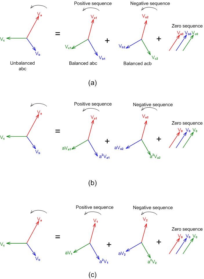
Figure 1 - Transformation from abc network to 012 sequence network
Knowing that multiplying a vector by will rotate it anti-clockwise by 90°, operators a and a2 to rotate a vector by 120° and 240°, respectively, are defined as:
Referring to Figure 1(a) and recalling that the positive and negative sequence networks are balanced, , all as shown in Figure 1(b). In a final step, the positive, negative and zero sequences are defined by the numerals 1, 2 and 0 respectively as shown in Figure 1(c). The transformation equations from the 012 sequence network to the abc network can now be written as shown in Figure 2.
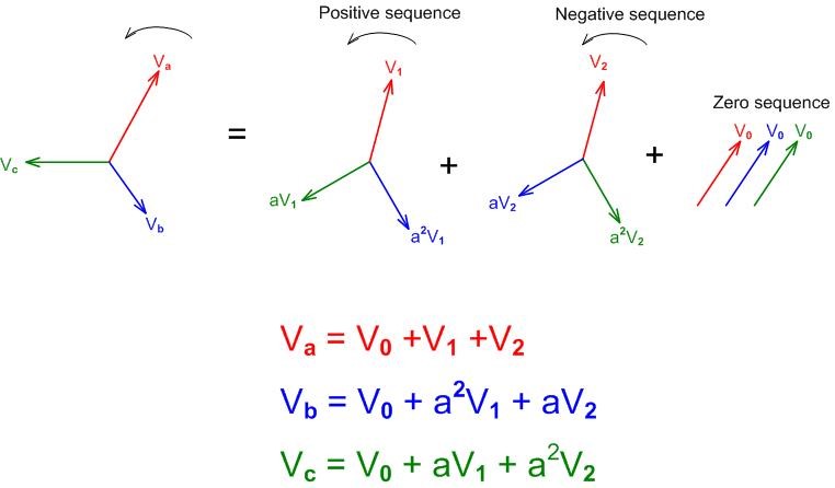
Figure 2 - Transformation voltage equations from abc network to 012 sequence network
The equations are usually expressed in matrix format
(1)
and the reverse transformation 012 to abc network equations are
(2)
Equations (1) and (2) are usually written in the short form using transformation matrices
giving
By substituting I for V in the equations the corresponding equations for current can be generated.
The sequence networks have actual circuit representation as shown in Figure 3 and are Thevenin equivalent networks as seen from the fault point. Each network has an impedance as shown but only the positive sequence network has a source voltage Vf which is the voltage at the fault point prior to the fault.
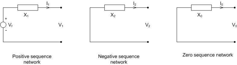
Figure 3 - Sequence networks
For calculations a consistent approach is recommended as follows below: draw the abc circuit for the case → write the equations for the case → make the transformation abc to 012 network → draw the 012 circuit and solve for the sequence voltages or currents as applicable → make the reverse transformation to give the abc solution.
3. Recovery Voltage Calculation: Fault Current Cases
3.1. General
The fault current interruption cases with respect to transmission and distribution circuit breaker standardized requirements include terminal faults, out-of-phase switching, short-line faults and double-earth faults. For out-of-phase switching the phase angle between the two systems is taken as 180° and the pole factor is 2 pu with no calculation necessary. Similarly the short-line fault is taken as a single-line-to-earth event and the pole factor for the system side voltage is 1 pu. Double-earth faults are applicable to circuit breakers on non-effectively earthed systems only.
3.2. Faults on Effectively Earthed Systems
The scenario for clearing a three-phase to earth fault is shown in Figure 4 where Va, Vb and Vc are phase voltages to earth. Initially all three phases carry the balanced fault.
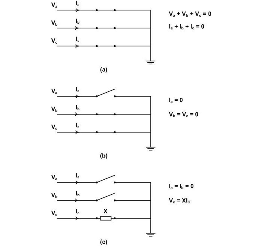
Figure 4 - Three-phase to earth fault current interruption in effectively earthed system
currents and no current flows to earth (Figure 4(a)). After current interruption in phase a, the first pole to clear, current continues to flow in phases b and c and to earth basically a double line to earth fault (Figure 4(b)). After current interruption in the second pole to clear, taken here as in phase b, current continues to flow in phase c as a single line to earth fault (Figure (c)). To calculate the pole factors for the first, second and third poles to clear, the following applies:
- Calculating the value Va in Figure 4(b) before the second pole clears will give the first-pole-to-clear factor.
- Calculating the value of Va or Vb in Figure 4(c) before the third pole clears will give the second-pole-to-clear factor which is also the first-pole-to-clear for a double line to earth fault.
- After current interruption in the third pole to clear, balance is restored and the third-pole-to-clear factor is unity.
3.2.1. First-Pole-to-Clear Factor Calculation
Referring to Figure 4(b) which also shows the abc network fault equations, the transformation to the 012 network is as follows the intent being to calculate the value of Va as a pole factor kpp1.
(3)
because
The sequence networks are connected in parallel as shown in Figure 5.
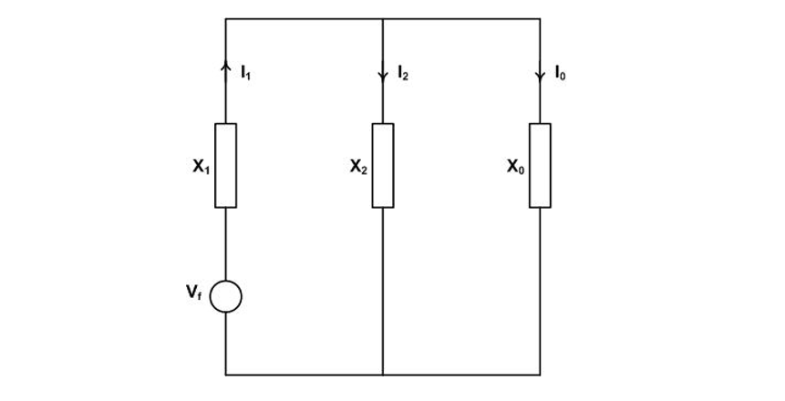
Figure 5 - Sequence network for the first-pole-to-clear recovery voltage calculation in an effectively earthed system
From Equation (3) and to Figure 3 for V1
For transmission system faults remote from balanced generation X2 = X1 and
(4)
For effectively earthed systems X0/X1=3 giving kpp1=1.2579 pu rounded up to 1.3 pu for circuit breaker standardization purposes [3].
3.2.2. Second-Pole-to-Clear Factor Calculation
Figure 4(c) shows the state after the first and second poles interrupt their respective fault currents leaving a single-line-to-earth fault on the third pole. The second-pole-to-clear recovery voltage will on the a and b phases and the task is to calculate Va and Vb while phase c still conducts fault current. Applying the transformation
The sequence networks are connected in series as shown in Figure 6.
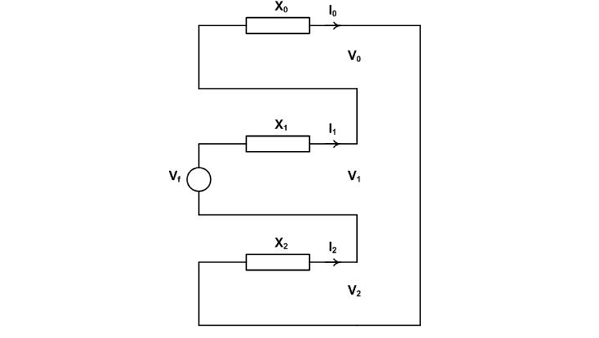
Figure 6 - Sequence network for the second-pole-to-clear recovery voltage calculation
(5)
(6)
(7)
Taking the reverse transformation
By substituting from Equations (5), (6) and (7), taking X2=X1 and repalcing a and a2 numerically, simple algebra yields the second-pole-to-clear pole factor kpp2.
Both quantities are equal in magnitude and kpp2 is calculated from the absolute values of each:
usually written in the form
For X0/X1 = 3, kpp2 = 1.2489 pu and rounded up to 1.26 for circuit breaker standardization purposes [3].
3.2.3. Third-Pole-to-Clear Factor Calculation
When the third-pole-to-clear interrupts the single line to ground fault current balance is restored and is demonstrated using symmetrical components as follows. In Figure 4(c), replace the pole in phase c with an impedance X (which ultimately goes to infinity) and the fault equation becomes
yielding the sequence equation
with the sequence network as shown in Figure 7.
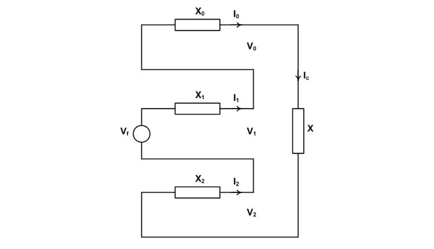
Figure 7 - Sequence network for the third-pole-to-clear recovery voltage calculation
Solving to Ic
3.3. Faults on Non-Effectively Earthed Systems
The three-phase fault prior to any current interruption is shown in Figure 8(a). Two cases are of interest: current interruption in the first-pole-to-clear, Figure 8(b), and current interruption in the second and third poles to clear, Figure 8(c). The second and third will interrupt in series sharing a recovery voltage equal to the line voltage.
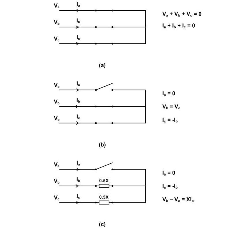
Figure 8 - Three-phase-fault current interruption in non-effectively earthed system
3.3.1. First-Pole-to-Clear Factor Calculation
Referring to Figure 8(b) and the abc network fault equations in particular
The sequence network connection is shown in Figure 9 noting that the zero sequence network does not exist in this case.
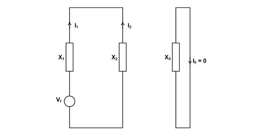
Figure 9 - Sequence network for the first-pole-to-clear recovery voltage calculation in a non-effectively earthed system
In the reverse transformation
(8)
This means that source side contribution is 1 pu because the system is balanced having no neutral. However, prior to current interruption in the second and third phases a voltage exists on the fault side of the first pole given by Vb or Vc. From Equation (8)
The voltage across the circuit breaker Vcb
and kpp1 for this case is
An early paper on recovery voltage calculation expressed the view that, taking X0 as infinity in Equation (4) which gives kpp1=1.5, covers this case [4]. This is not correct and is discussed further in the appendix.
3.3.2. Second and Third Pole-to-Clear Factor Calculation
Referring to Figure 8(c), the recovery voltage is calculated by replacing the circuit breaker poles in phases b and c with impedances 0.5X.
Making the transformation
Likewise
The calculations indicate a sequence network as shown in Figure 10. Taking X1 = X2.
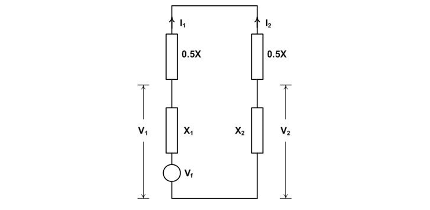
Figure 10 - Sequence network for the second and third pole-to-clear recovery voltage calculation in a non-effectively earthed system
From the fault equations
The recovery voltage for each pole will be
3.3.3. Double-Earth Fault Recovery Voltage Factor Calculation
A double-earth fault is a variation of a line-to-line fault the difference being that the fault between the lines is through earth. The difference is illustrated in Figure 11. Only the phase b circuit breaker pole will carry the fault current and the recovery voltage will be 1.73 pu due to the sustained earth fault on phase a.
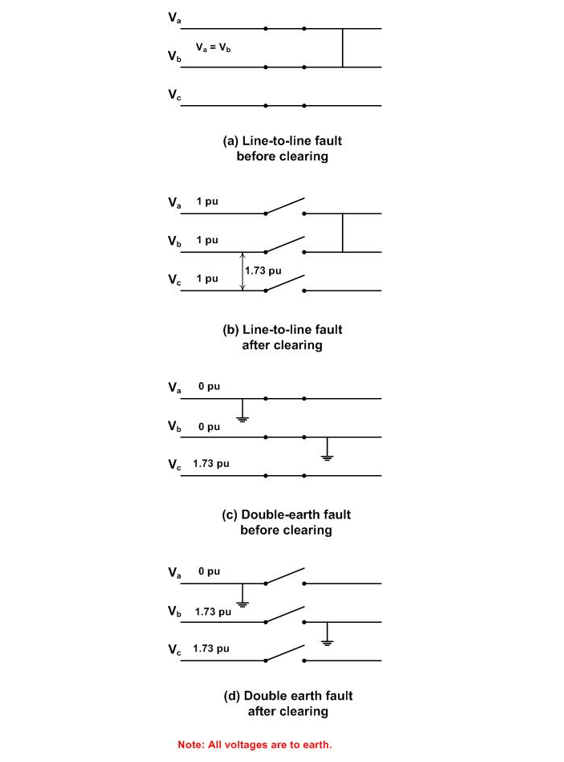
Figure 11 - Faults in non-effectively earthed systems involving two lines: line-to-line fault (a) before current interruption and (b) after current interruption; double-earth fault (c) before current interruption and (d) after current interruption
4. Inductive Load Current Switching
Inductive load current switching covers the cases of motor switching and shunt reactor switching [3, 5]. Only the latter switching case is relevant for the topic of this paper.
The general case for shunt reactor switching is shown in Figure 12 where L is the reactor inductance, LN the neutral reactor inductance and CL the total load side capacitance.
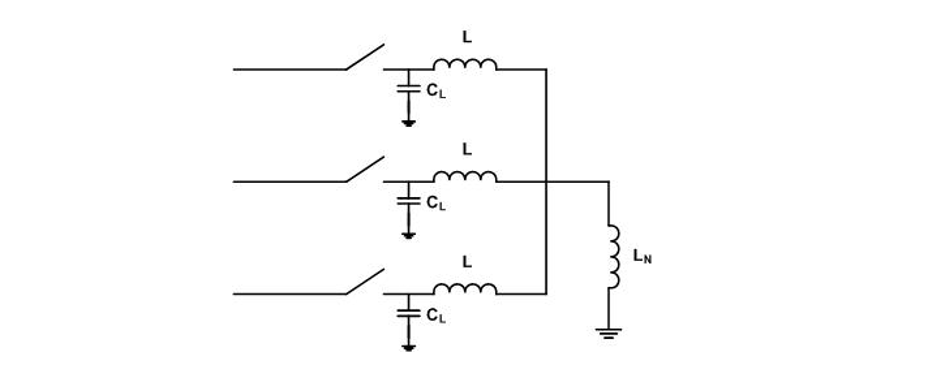
Figure 12 - General circuit for shunt reactor switching
The first-pole-to-clear representation is shown in Figure 13(a) which simplifies to that in Figure 13(b) and finally to that in Figure 13(c) where K is the neutral shift as indicated.
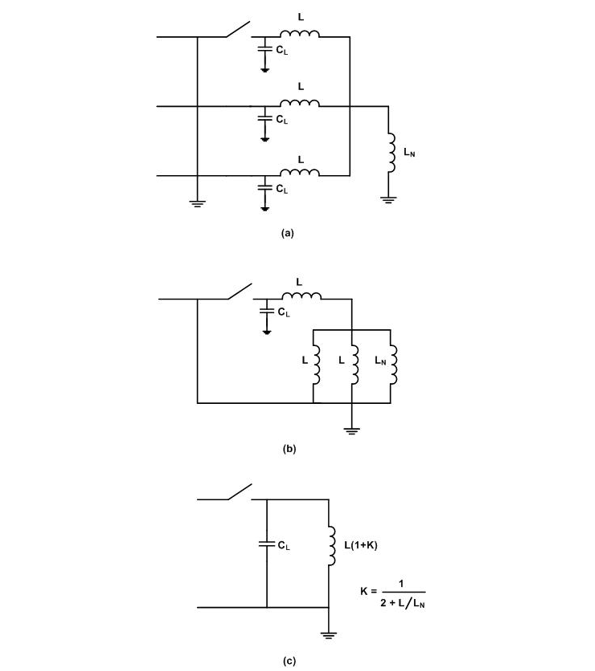
Figure 13 - First-pole-to-clear circuit representation
This is load current switching and the system side contributes 1 pu and any excursion above that comes from the load circuit configuration to give a pole factor of 1+K. For the earthed neutral and non-earthed neutral cases, the pole factors are 1 pu and 1.5 pu, respectively, and, for the neutral reactor earthed cases to enable single-pole fault clearing and high-speed reclosing, the pole factor is typically around 1.3 pu.
For reactors with non-earthed neutrals, the axis of oscillation for the TRV across will be the shifted neutral adding two times K, i.e. 1 pu voltage, to the TRV peak. This is a serious consideration in the choice of the circuit breaker rated voltage for the purpose. By way of example Figure 14 shows the TRVs for a 30 kV 100 Mvar with an earthed and non-earthed neutral.
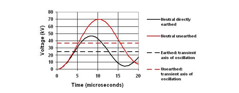
Figure 14 - Switching out at 30 kV, 100 Mvar reactor with earthed and non-earthed neutral
The consideration of shunt reactor switching pole factor calculation can be extended to treat the addition of series reactors to limit fault current levels. Such reactors are essentially low impedance shunt reactors under fault conditions. The general circuit and equations for pole factor calculation is shown in Figure 15 where the reactor impedance is designated as X and the neutral impedance as Xe. The intent is to calculate the equations for Va and Ve in pu.
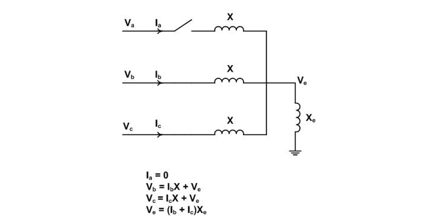
Figure 15 - General circuit for shunt reactor switching first-pole-to-clear factor calculation
The transformation from the abc network to the 012 network yields the sequence network shown in Figure 16.
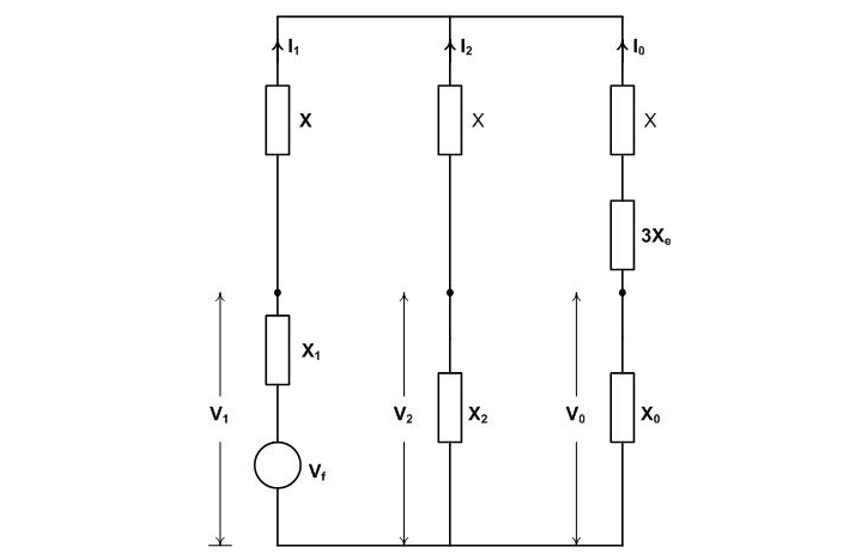
Figure 16 - Sequence network for calculation of first-pole-to-clear for shunt reactor switching
The calculation to determine Va /Vf and Ve /Vf and the resulting equations are [5]:
(6)
For an infinite and balanced system, the positive sequence and negative sequence impedances can be taken as zero and the reader can verify that Va /Vf=1 and Ve /Vf is that determined in the simpler calculation in Figure 13.
As noted earlier the above treatment of shunt reactor switching is valid for series reactors under fault conditions. The latter case is however more complex because the source now delivers a TRV dependent on the distribution of the recovery voltage between the source and reactor impedances.
For the case of a three-phase fault in an effectively earthed system, setting Xe = 0 in Equation 9 gives the pole factor kpp as
and replacing X0=3X1 yields kpp as a function of the ratio X / X1:
(10)
Equation 10 is plotted in Figure 17.
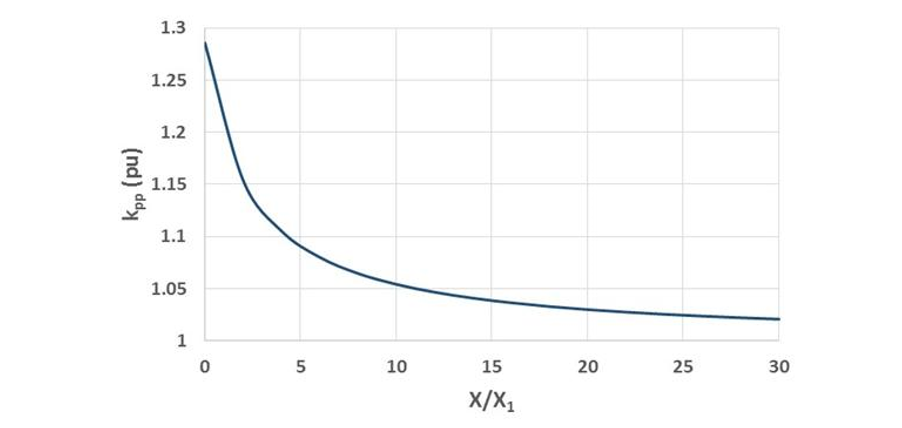
Figure 17 - Plot of pole factor for series reactor limited faults in effectively earthed systems
Note that for X = 0, kpp = 1.2857 pu as expected. As a further test, as X1 decreases, relative to X approaching zero for the shunt reactor switching, then the equation should yield kpp = 1 and the reader can verify that this is the case.
5. Capacitive Load Current Switching
Capacitive load current switching covers the case of shunt capacitor bank switching and the switching of unloaded transmission lines and cables. Starting with the unloaded line case, the lines have phase-to-earth capacitance CE and phase-to-phase capacitance CL as shown in Figure 18.
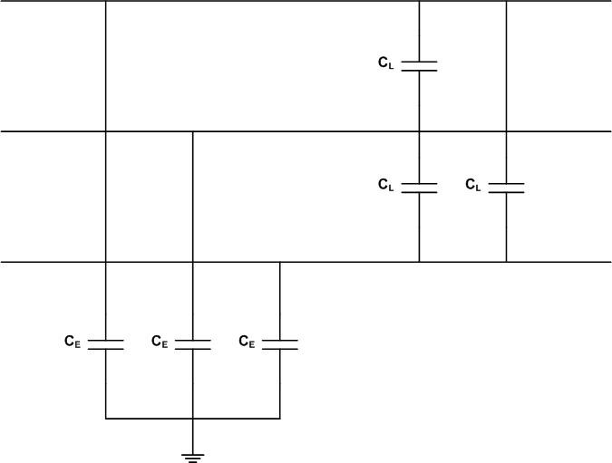
Figure 18 - Basic transmission line circuit representation
The equation for the phase line charging current I for a phase-to-earth voltage V is:
A delta-to-wye conversion of the line-to-line capacitances converts the circuit in Figure 18 to that shown in the upper part of Figure 19. To derive the sequence network
and thus
and the network is as shown in the lower part of Figure 19.
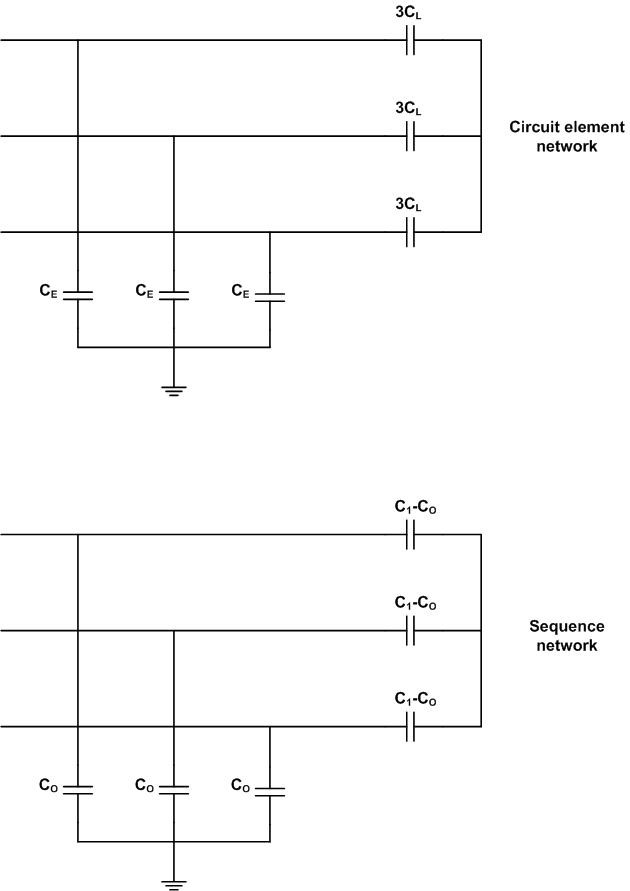
Figure 19 - Transmission line circuit element network and sequence network
The pole factor kpp is readily calculated similarly to that for the shunt reactor switching case and is given by [5]:
and is the voltage to be applied in a test circuit to achieve the correct recovery voltage krv of 2 pu after current interruption as given by:
The equations for kpp and krv are plotted in Figure 20.
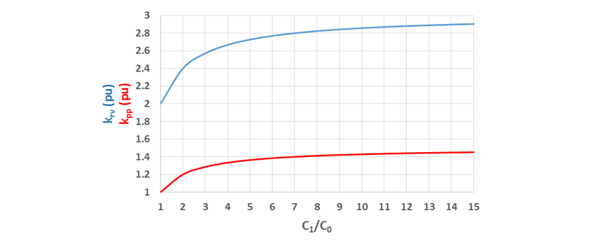
Figure 20 - Pole factor kpp and recovery voltage factor for krv as a function of C1 ⁄ C0
A detailed description of capacitive current switching and the application of Figure 20 to the different cases noted earlier can be found in [3].
6. Conclusion
The intent of this paper is to cover the detailed calculation of pole factors across the range of fault current cases in effectively and non-effectively earthed power systems and also as they relate to inductive and capacitive load current switching. The calculations, taken together with the TRV oscillatory component calculations described in [1], provide a complete analytical approach to TRV calculation.
References
- D.F. Peelo, “Generalized Approach to Analytical Circuit Breaker Transient Recovery Voltage Calculation,” CSE 025, June 2022.
- C.L. Fortescue, “Method of Symmetrical Coordinates Applied to the Solution of Polyphase Networks,” AIEE Transactions, June 1918.
- IEC 62271-306: High-Voltage Switchgear and Controlgear – Part 306: Guide to IEC 62271-100, IEC 62271-1 and Other IEC Standards Related to Alternating-Current Circuit Breakers.
- R.H. Park and W.F. Skeats, “Circuit Breaker Recovery Voltages: Magnitudes and Rates of Rise,” AIEE Transactions, Volume 50, Issue 1, 1931.
- D.F. Peelo, “Current Interruption Transients Calculation,” John Wiley & Sons, January 2020.
Appendix: Historical Notes
The state of electrical circuit analysis prior to 1918 is described in an article by R.D. Barnett [A1]. No method existed to deal with unbalanced three-phase circuits until the publication of the classic paper by C.L. Fortescue of Westinghouse in 1918 [A2]. The paper is the longest ever published by the AIEE/IEEE at 114 pages, 88 pages to the paper itself and 24 pages of discussion. The paper does not specifically address three-phase power systems but rather general n‑phase systems and is a complex read. However, the main discusser, J. Slepian also of Westinghouse, captured the essence of the method as it applies to three-phase systems introducing the notion of positive, negative and zero sequence representation (see pages 1117-1118 of [A2].
At that time fault current interruption and recovery was viewed on a rated voltage and current magnitude (kVA) basis. The idea that higher recovery, perhaps even with higher frequency transients, might exist came in 1927 in a comment by J.D. Hilliard of General Electric (GE) in a comment to a paper that read [A3]:
“…the difficulty in interruption depends largely upon the magnitude of the voltage ‘kick’ at the end of each half wave of the arc, and upon the speed at which each half wave of transient voltage is built up”
representing the first recognition of transient recovery voltages (TRVs). GE followed up with actual testing to verify and measure actual AC recovery voltages [A4]. The paper, authored by W.F. Skeats and R.H. Park was the first step leading to the first standardized TRVs in the 1950s. (Note: R.H. Park is best known for his contributions to synchronous machine theory.)
Figure A1 shows an extract from [A4] which is probably the first publication of the equation for the pole factor for the first-pole-to-clear for a three-phase-to-earth fault in an effectively earthed power system.
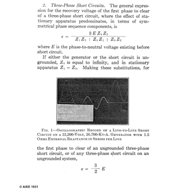
Figure A1- Excerpt from Reference [A4] first-pole-to-clear equation for three-phase to ground fault on effectively earthed system
The paper also includes detailed calculation of the above pole factor and additionally that for first pole clearing for a double-line to earth fault using symmetrical component theory. However, with reference to Figure A1, the claim is made that the equation is valid for the first-pole-to-clear for a three-phase fault on a non-effectively earthed system by taking the zero sequence impedance Z0 as being equal to infinity. Calculation of this quantity in the main text showed that Z0 does not exist for this case and cannot be assigned a value other than zero (refer to Figure 9). Why then does setting give a supposedly correct result at 1.5 pu?
Figure A2 shows the general circuit enabling first-pole-to-clear calculation for three-phase faults on both effectively and non-effectively earthed systems.
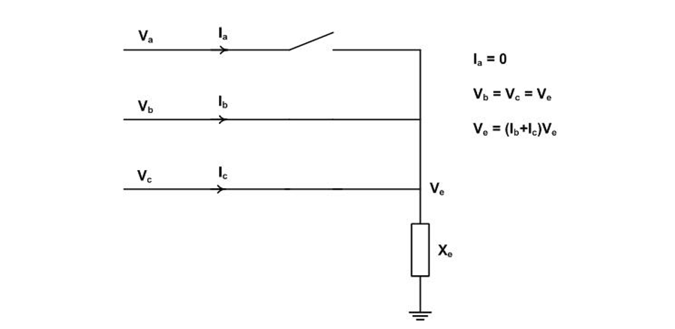
Figure A2 - General circuit for first-pole-to-clear for three-phase faults in effectively and non-effectively earthed systems
For the former case and for the latter
and
. Taking
and
covers the claim made in paper (Figure A1). Calcuation of Va and Vb yields the results shown in the table below.
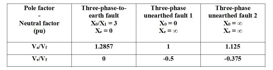
General first-pole-to-clear calculation results
The claim calculation ironically does give 1.5 pu across the circuit breaker, however the source and neutral side values of 1.125 pu and 0.375 pu, respectively, are not possible in reality. The claim is therefore false and may have its origin in an assumption that, if I0 = 0, then Z0 can be taken as being infinite.
A number of textbooks were published in the 1930s and 1940s, the most notable and practical of those were by C.F. Wagner and R.D. Evans of Westinghouse and E. Clark of GE [A5, A6]. Both of these books provide calculation of the recovery voltages for the cases discussed in the main text above. Note that the term pole factor did not come into common use until the first circuit breaker standards were developed in the 1950s.
With respect to technical journal references, the first AIEE paper specifically on unbalanced fault voltage and current calculation is that of R.D. Evans and S.H. Wright of Westinghouse [A7]. A study from 1946 by P. Hammarlund of ASEA, Sweden is frequently referenced due, at least in part, to its citation and quotation at length in the well-known 1971 textbook by A. Greenwood of GE [A8, A9]. The study is actually on TRV calculation and only a very minor part is given over to recovery voltage calculation. Hammarlund takes the case of the first-pole-to-clear for a three-phase fault on an effectively earthed system and proposes replacing the breaker by an impedance Z, completing the calculation and in ultimate allowing Z to go to zero. Two excerpts from the study are shown in Figure A3.
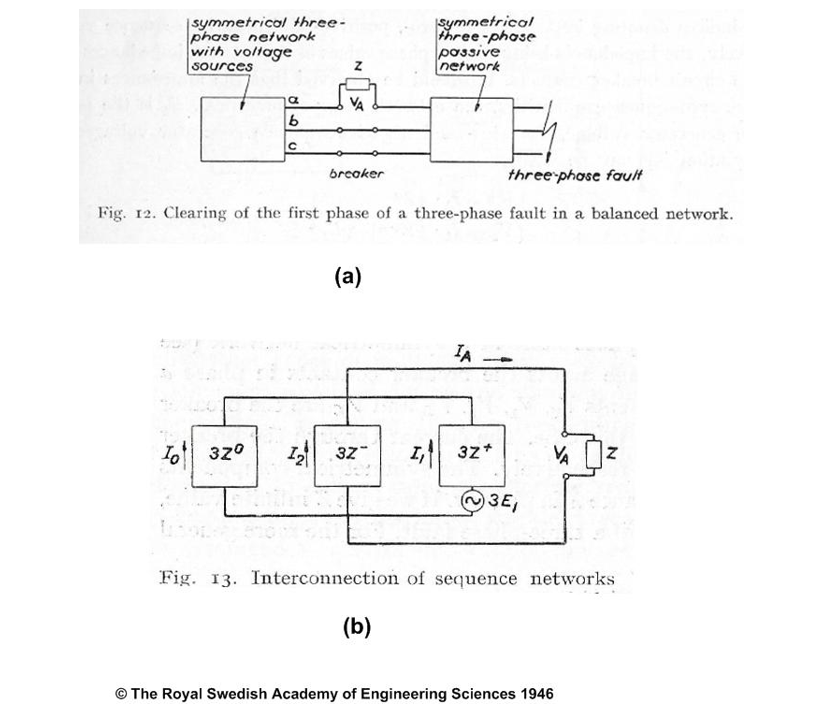
Figure A3 - Excerpt from Reference [A8]: (a) System fault scenario and circuit breaker first-pole-to-clear representation; (b) Sequence network for first-pole-to-clear
The first excerpt, Figure A3(a), shows the proposal at a system level and the second excerpt, Figure A3(b), the derived sequence network for the case. The sequence network is correct but curiously neither author completes the calculation to fruition despite Hammarlund citing [A4] a textbook by W. Lyon (see Further Reading) and Greenwood [A5] and [A6] as references. To complete the calculation, the fault equations of Figure 4(b) apply except that now Va = IaX.
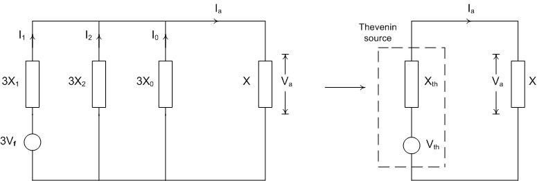
Figure A4 - Sequence network conversion to Thevenin equivalent circuit
Referring to Figure A4 showing the sequence network and the Thevenin equivalent circuit and taking X1 = X2, the Thevenin voltage Vth is given by:
and the pole factor is
The proposal works for this case and, as shown in the main text, is of value for other cases, refer to Figures 4(c) and 8(c).
Suggestion for further reading can be found after the references.
Appendix References
A1. R.D. Barnett, “Short circuit protection: Challenges in the early years,” IEEE Power & Engineering Journal, Volume 19, Number 4, July/August 2021.
A2. C.L. Fortescue, “Method of Symmetrical Coordinates Applied to the Solution of Polyphase Networks,” AIEE Transactions, June 1918.
A3. P. Sporn and H.P. St. Clair, “Tests on High and Low-Voltage Oil Circuit Breakers,” AIEE Transaction 46, 1927.
A4. W.F. Skeats and R.H. Park, “Circuit Breaker Recovery Voltages – Magnitudes and Rates of Rise,” AIEE Transaction 50, 1931.
A5. C.F. Wagner and R.D. Evans, “Symmetrical Components: As Applied to the Analysis of Unbalanced Electrical Circuits,” McGraw-Hill Book Company Inc., 1933.
A6. E. Clarke, “Circuit Analysis of AC Power Systems,” John Wiley & Sons, Inc., 1943.
A7. R.D. Evans and S.H. Wright, “Some Effects of Unbalanced Faults,” AIEE Transactions Volume 50, Issue 6, June 1931.
A8. P. Hammarlund, “Transient Recovery Voltage Subsequent to Short-Circuit Interruption with Special Reference to Swedish Power Systems,” Proceedings No. 189, Royal Swedish Academy of Engineering Sciences, 1946.
A9. A. Greenwood, “Electrical Transients in Power Systems,” John Wiley & Sons, Inc., 1971.
Further Reading
- W. Lyon, “The Method of Symmetrical Components,” McGraw-Hill Book Company, Inc., 1937.
- Electrical Transmission and Distribution Handbook (Chapter 2), Westinghouse Electric Corporation, 1964.
- J.L. Blackburn, “Symmetrical Components for Power Systems Engineering,” Marcel Dekker, Inc., 1993.
- P.M. Anderson, “Analysis of Faulted Power Systems,” Wiley-IEEE Press, 1995.
- N. Tleis, “Power System Modelling and Fault Analysis (Chapter 2),” Newnes, 2008.
Biography
David Peelo is a graduate of University College Dublin and Eindhoven University of Technology. He is a former switching specialist at BC Hydro and is now an independent consultant. He is an IEEE Distinguished Lecturer and a Distinguished Member of CIGRE and is a former chair of the Canadian National Committee for IEC Technical Committee TC 17 and Subcommittees 17A and 17C. He is the author of a textbook on transient recovery voltage calculation and the coauthor of two other textbooks on switchgear and switching including a CIGRE Green Book.