Enhanced Real-Time Multi-Terminal HVDC Power System Benchmark Models with Performance Evaluation Strategies
Authors
A. SHETGAONKAR, M. POPOV, A. LEKIĆ- Delft University of Technology, Faculty of Electrical Engineering, Mathematics and Computer Science, Delft, The Netherlands
T. KARMOKAR - Delft University of Technology, Faculty of Electrical Engineering, Mathematics and Computer Science, Delft, The Netherlands - TenneT TSO GmbH, Germany

Summary
Real-time simulations have become a crucial tool for life cycle studies of VSC-based HVDC systems. This paper introduces real-time Multi-Terminal HVDC (MTDC) power system network models[1] with real-time wind profile feedback. It addresses the shortcomings of existing benchmark network models and fills the modeling gaps. RSCAD®/RTDS environment represents the real-time modeling techniques for studying the life cycle of Bipolar Metallic Return configuration of HVDC systems. This paper evaluates the performance of the proposed network model using unscheduled events, startup, and black start events. Future studies can be conducted using the proposed network models by mimicking the actual performance of cable-based DC grids while considering the computational insights from this paper. The findings of this paper shall enable the identification of various stress points that can be utilized to specify technical requirements for component design and AC/DC protection studies concerning startup and black start sequence.
Keywords
Multi-Terminal DC, Metallic Return, AC/DC Protection, RTS model, SILNomenclature
HV High Voltage
HVDC High Voltage Direct Current
TSO Transmission System Operator
VSC Voltage Source Converters
EMT Electromagnetic Transient
DC CB Direct Current Circuit Breakers
RTS Real-Time Simulator
DMR Dedicated Metallic Return
MTDC Multi-Terminal (HV) DC
VARC Voltage-source converter Resonant Current
MMC Modular Multilevel Converter
HIL Hardware-in-the-loop
SIL Software-in-the-loop
RSCAD®/RTDS Real-Time Digital Simulator
SM Sub-Module
HB Half-Bridge
SLG Single Line to Ground fault
OVC Outer Voltage Control
ICC Inner Current Control
LCC Lower Level Control
PLL Phase Lock Loop
DVC Direct Voltage Control
CCSC Circulating Current Suppression Control
PCC Point of Common Coupling
GSC Grid-Side Control
MSC Machine-Side Control
TCP/IP Transmission Control Protocol/Internet Protocol
PMSM Permanent Magnet Synchronous Machine
PG Pole to Ground fault
1. Introduction
Over the last two decades, the demand for real-time simulations using EMT software and HIL has increased significantly. Real-time simulators (RTSs) are commonly used for various purposes, including testing new or refurbished HVDC projects, post-disturbance and failure analyses, investigating HVDC and AC system interaction, and studying HVDC special emergence protection schemes. Extensive studies and systematic libraries have been performed and published in that direction. The most recent CIGRE 804 [1] brochure provides RSCAD® /RTDS average value MMC models for 500kV voltage levels. The benchmark models represent the overhead DC transmission. As a part of the PROMOTioN project, deliverable D9.1 provides a three-terminal grid model with ±320 kV rated DC voltage [2]. The main task of real-time simulations is to perform detailed multivendor studies that simulate near real-time situations. So far, there have been realized multivendor protection studies [3].
Furthermore, Best Paths [4] and PROMOTioN [2] projects provide a reasonable basis for the multivendor control and protection studies, which are currently being extended by READY4DC and InterOPERA projects. Offshore wind farms are connected to the converter station, which can be intertwined with the controller’s frequency range, and therefore control system needs to be modeled in detail. This captures the possible offshore control interaction. To ensure equipment safety and system stability in the offshore HVDC islanded operation, voltage stability studies must be carried out with the coordination of wind farm control and frequency stability. Furthermore, the interaction of the interwind turbine and stability control in HVDC islanded operation requires a detailed representation of offshore wind farms in the RTS. However, for studies on harmonic stability, frequency domain methods can be used iteratively using the script functionality of RTS. Thus generally, RTS is important to benchmark the control system and model used. Besides, from the system owner’s perspective, avoiding the system risk of instability or tripping of the connected AC submarine cable in the case of short circuit faults during offshore HVDC islanded operation is a crucial techno-economical factor. Planned projects in the north sea focus on ±525 kV DC voltage with a DMR and a bipolar topology. Hence, the impact of DMR cable on the HVDC grid and vice versa will be crucial during the energization, the transient event, and the post-disturbance state. To investigate these, a phase domain frequency-dependent model of DMR with realistic data and modeling techniques is required.
To increase the reliability of offshore wind power, the North and Baltic Sea TSOs are considering the implementation of direct current circuit breakers (DC CB) breakers in the HVDC grids. However, many technical and economical challenges; have been analyzed, and solutions are provided in the PROMOTioN project. The operation of DC CBs on system components like converter and cables needs to be investigated during energization, as well as the DC fault and breaker re-close period. The time simulation studies during this period will provide input for design and operation studies.
This paper provides RTS models for the point-to-point, three-, four- and five-terminal HVDC grids. These models are developed by applying the guidelines established in the recent CIGRE brochures [5, 6] and filling up the gap that needs to be covered by recent CIGRE brochures [1, 7]. These models are available as open software for future users [8]. The ratings of the upcoming ±525 kV, 2 GW offshore aggregated wind farm connections with DC CB have been used in their design. Per [5], path B is considered in this work, as shown in Figure 1, and aims to increase the application of the developed model for academic and industrial projects. Some of the primary key features of the developed network over existing benchmark models are the interfaced aggregated wind turbine model, scripted parameters, simplified VARC DC CB model, DMR cable model, easy expandability, and Real-time wind profile [8]. Similarly, this work provides insight into the computation requirement for real-time simulations.
The proposed model closes the following modeling gap in the benchmark network:
- Proposed network models consist of ±525 kV Submarine and land cables.
- Proposed network models consider wind farm/wind turbine dynamics based on Real-time wind gusts using SiL setup.
- Electrical and Control parameter perturbation using an automatic script.
- Provides an overview of required cores per network models.
- Proposed networks consist of an average model of VARC DC CB.
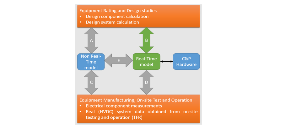
Figure 1 - Different validation paths overview during the HVDC project phases [5]
2. Network Description
For the interoperable control and protection studies, the Multi-terminal DC (MTDC) power system should be designed with the maximum amount of details. In this paper, different MTDC configurations will be considered depicted in Figure 2.
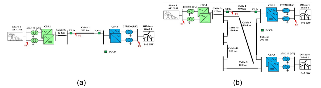
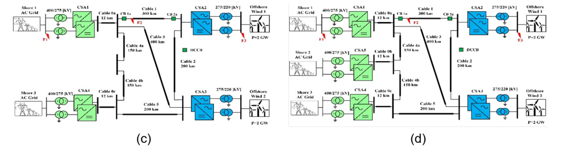
Figure 2 - MTDC with (a) two terminals; (b) three terminals; (c) four terminals; and (d) five terminals
The network topologies have a DC voltage rating of ±525 kV, with bipolar dedicated metallic return (DMR) configurations. The converter is a half-bridge topology. The system can be divided into three subsystems: the onshore AC system, the DC system, and the offshore AC system.
The onshore AC system consists of Thevenin’s equivalent circuit (static voltage source) of a strong grid; the grid impedance is computed based on the short circuit current level—a series resistor connection of a parallel resistor and inductor models it. By adjusting the values of the inductance and resistance, the short circuit current value and the damping angle at fundamental and Nth harmonic are controlled.
The rated line-to-line (LL) voltage is 400 kV. The onshore converter station has two Y-D transformers, with ratings of 2 GVA each. The voltage ratio of this transformer is 400 kV/275 kV. Onshore converters are labeled CSA1, CSA4, and CSA5. However, based on the selected topology, the converters are omitted.
The number of land and submarine DMR cables varies depending on the network topologies. For the five-terminal HVDC system, the number of land DMR cables are Cable 0a, 0b, and 0c. The length of these cables is 12 km. The land cables connect the onshore DC hub, which comprises DC breakers; for simplicity and to reduce the computation burden, only one DC breaker is employed. Furthermore, the DC system comprises six submarine cable links: cable 1 (300 km), cable 2 (200 km), cable 3 (400 km), cable 4a (150 km), cable 4b (150 km), and cable 5 (200 km). The cables are modeled as a frequency phase-depended model. Furthermore, the cable link consists of three conductors (i.e., a positive, a negative cable, and metallic return per cable link) due to DMR topology. Cable 1 consists of two simplified VARC DC CB placed on the positive pole at either end of the cable, as seen in Figure 2.
The offshore AC system consists of converter stations and aggregated average-value model wind farms. In the applied networks, offshore converters are labeled CSA2 and CSA3. However, based on the topologies, the converters are omitted. The offshore converter is connected to the offshore AC system via D-Y transformers. The rating of this transformer is 275 kV/220 kV, 2 GVA. Besides, this converter transformer is connected to a wind turbine transformer. This transformer has a voltage ratio of 220 kV/66 kV and acts as a VA scaled-up transformer. Thus, a power rating of 2 GW can be achieved by choosing the proper scaling factor. The lower voltage end of this transformer is connected to the wind turbine. The wind turbines are type 4 and have a rating of 2 MW at a wind speed of 15 m/s. In this work, three fault locations are selected. F1 indicates an AC fault at the Point-of-Common Coupling (PCC) of the CSA1, F2 indicates a DC fault at the DC terminal near CSA1, and F3 indicates an AC fault at the PCC of CSA2.
2.1. Converter station
In each network topology, the converter station per pole (i.e., positive and negative pole) comprises four key elements: converter transformer, startup insertion resistor, arm reactor, and valve, as shown in Figure 3. The converter transformer is a two-winding, star-delta configuration. A tertiary winding may provide auxiliary power to the converter station from the AC system. However, in this study, the tertiary winding is absent. The AC grid side is connected to the transformer’s star side, and the DC grid side to the delta side. The delta connection prevents the low-frequency zero-sequence voltage from being injected into the AC system.
Furthermore, the leakage inductance of the transformer and the arm rector provide sufficient reactance between the AC-side voltage and the valve required to control the AC grid current. Due to the near-pure sinusoidal waveform of the converter’s voltage, a standard AC transformer is adopted. This transformer also provides galvanic isolation between the AC and DC grids.
The pre-insertion resistors are placed between the AC bus and the converter transformer. To limit the inrush current produced by charging the sub-module (SM) capacitors, DC filters, DC line/cable, and the remote station, the resistor is switched on for a few seconds and bypassed after a dedicated set period. The arm reactor is connected in series with a converter valve. In this work, the arm reactor is placed on the AC side of the converter. The arm reactor limits the circulating current between the converter valves.
Furthermore, it also limits the rate of rise of the fault current. Each converter valve consists of n SMs. In the presented networks, the number of SMs is selected based on the geographical location. For the studied cases, a half-bridge (HB) topology of the SM is selected, which consists of three main states: Bypass, Blocked, and Inserted state. However, the voltage across the SM is determined by the current direction.
| Parameter | Onshore converter station per MMC | Offshore converter station per MMC |
|---|---|---|
Rated Power | 2000 MVA | 2000 MVA |
fundamental frequency | 50 Hz | 50 Hz |
AC grid voltage | 400kV | 220 kV |
AC converter bus voltage | 275 kV | 275 kV |
DC link voltage | 525 kV | 525 kV |
Transformer reactance | 0.18 pu | 0.15 pu |
MMC arm inductance | 0.025mH | 0.0497mH |
MMC arm resistance | 0.0785 | 0.0785 |
Capacitor energy in each submodule (SM) | 30 MJ | 30 MJ |
Number of submodules per valve | 240 | 200 |
Rated voltage and current of each submodule (SM) | 2.5 kV /2kA | 2.5 kV / 2kA |
Conduction resistance of each IGBT/diode | 5.44‧10-4 | 5.44‧10-4 |
With the high number of SMs, the AC side of the valve provides a smooth AC waveform. The Type 5, i.e., Average Value Models (AVM) [9] based on switching functions, converter model is used in these networks. To capture the accurate dynamics of the converter station, it is modeled by using small time steps of RTDS. Table I lists the converter station parameters with associated values used in this work. Further, to reduce the tedious modeling time, control, electrical parameters, and limits values are scripted using draft variables. These draft variables are controlled via a script at the start simulation. This script is written in C++ in an RSCAD®/RTDS environment.
2.2. HVDC Cable
HVDC cables enable bulk power transmission over long distances without charging the transmission line’s capacitance with alternating voltage. This makes HVDC a lucrative and highly efficient option for power transfer. The compact transistor-based Voltage Source Converter (VSC) technology results in the absence of the need to change voltage polarity for reversal of power direction. This has made extruded insulation the preferred choice for HVDC cable systems. Reverse voltage polarity causes superposition of transient stresses on steady-state DC stress, which could be detrimental to the performance of the extruded insulation due to the presence of space charges and consequent localized increase in the electric stress. Extruded insulation makes the cable manufacturing process, relative to oil-impregnated paper insulation, faster, more cost-effective, and environmentally friendly. Extruded insulation with cross-linked polyethylene (XLPE) has now been serviced at up to 400 kV [10]. The qualified voltage level of extruded cables is 640 kV [11]. The present clean energy transition in Europe [12], which aim to integrate maximum offshore wind into the electrical grid [13] along with land-based energy highways that are currently being implemented in Germany [14], all make use of extruded insulation systems, primarily based on XLPE technology at 525 kV.
The performance of DC cables in service is strongly governed by their electric conductivity, which defines the distribution of the electric field under DC voltage. As the cable carries the load current, joule heating of the conductor creates a temperature gradient over the entire thickness of the cable insulation. This temperature drop is a specified design value for a particular DC extruded insulation. It is verified for the cables in long-term qualification and design-verification tests with its joints and termination. This way, the cables and their electrical interface with associated cable accessories are tested and qualified. Additional insulation heating might result from the leakage current through the insulation due to the electric stress. The leakage current is a characteristic phenomenon that plays a decisive role in demonstrating the electrical integrity of the extruded DC cable insulation system as it quantifies the dielectric loss. The effect is cyclic as the increased temperature of the insulation would increase its losses, which will further increase its electrical conductivity. Such sequential events can lead to thermal runaway if the conductivity exceeds the upper limit’s threshold. In DC, the pattern in the electrical field distribution is controlled by temperature-dependent conductivity. The highest electrical stress is encountered near the cable screen at high loads, whereas at no loads, it is near the conductor. In this work, these factors have been considered in cable modeling. As described in the previous section, sea, and land DMR cables are considered. The cable is modeled using Frequency Dependent (Phase) model. The data for the cable model is based on the experience of 2 GW [13] Offshore Interconnection projects in the North Sea and has been listed in Tables II and III.
| Main layers | Properties | Unit | Parameter Data (Nominal) |
|---|---|---|---|
Core Conductor | Metallic cross-sectional area | [mm2] | 3000 |
Outer diameter | [mm] | 68 | |
DC resistivity (max.) at 20°C | [Ωm] | 1.7241‧10-8 | |
Main Insulation (XLPE) | Conductor Screen thickness | [mm] | 1.8 |
Main insulation thickness | [mm] | 26.5 | |
Insulation screen thickness | [mm] | 1.5 | |
Relative permittivity | - | 2.4 | |
Metallic Screen | Screen thickness | [mm] | 1.2 |
Diameter over screen | [mm] | 138 | |
DC resistivity (max.) at 20°C | [Ωm] | 2.8264‧10-8 | |
Outermost Jacket | HDPE Jacket Thickness | [mm] | 5.0 |
External semiconductive skin thickness | [mm] | 0.3 | |
Relative permittivity | - | 2.5 | |
Overall cable | Diameter | [mm] | 153 |
| Main layers | Properties | Unit | Parameter Data (Nominal) |
|---|---|---|---|
Core Conductor | Metallic cross-sectional area | [mm2] | 2500 |
Outer diameter | [mm] | 60 | |
DC resistivity (max.) at 20°C | [Ωm] | 1.7241‧10-8 | |
Main Insulation (XLPE) | Conductor Screen thickness | [mm] | 2.0 |
Main insulation thickness | [mm] | 26.0 | |
Insulation screen thickness | [mm] | 1.8 | |
Relative permittivity | - | 2.4 | |
Metallic Sheath | Material | - | Lead |
Thickness | [mm] | 3.2 | |
DC resistivity (max.) at 20°C | [Ωm] | 2.14‧10-7 | |
Armour | Material of Armour wires | [mm] | galvanized steel |
The thickness of single armor wire | [mm] | 6.0 | |
Overall cable | Diameter | [mm] | 161 |
2.3. Direct Current Circuit Breaker (DC CB)
Among the many different DC CB technologies, voltage-source converter resonant current (VARC) DC CB technology is selected for these networks. The VARC DC CB uses a voltage source converter (VSC) and a series-resonant circuit to generate high-frequency current oscillation, which creates a current zero in the Vacuum interrupter. The VARC DC CB consists of three major branches, i.e., a main, energy absorption, and current injection branch, as shown in Figure 4(d). Furthermore, the working principle, experimental validation, and modularity of the DC CB are explained in [15]. Furthermore, the advantage of this average model is that it can be modeled using power system components of the RSCAD® library with no dedicated core requirement.
Figure 4 - Equivalent Average Model of VARC DCCB model
Factors contributing to the selection of load units and limits are memory requirements, the number of computations, and execution speed. However, the main aim of the design model is to keep the time-step at a reasonable size for real-time simulation. Thus, an equivalent average model of VARC DC CB is proposed in [16]. Hence, this work adopts an equivalent average model of a VARC DC CB for system-level dynamic studies. Like the detailed VARC DC CB, the equivalent average model consists of three branches. During the operation of VARC DC CB, these branches are connected in series for Nm modules, as shown in Figure 4(a-c). As a result, an aggregation of the VARC parameter is possible, as shown in Figure 4(d). Parameters for each branch are aggregated for the rated DC-link voltage, and aggregated values are shown in Table IV.
| Parameters | Symbol | Detailed model | Average model |
|---|---|---|---|
Oscillation Inductor | Lp | 95 μH | 0 μH |
Oscillation Capacitor | CP | 2.72 μF | 0.388 μF |
Rated / clamping voltage | Vrated /Vclamp | 80/120 kV | 525/787.5 kV |
Initial voltage across CP | 10 kV | 0 kV | |
Number of modules | Nm | 7 | 1 |
2.4. Wind Turbine/Plant Model
The Wind Turbine model used for this study is a Type 4 model [17], with a single-line diagram shown in Figure 5. The Type 4 wind turbine model consists of four main components: the Wind turbine model, a permanent magnet synchronous machine (PMSM), an AC-DC-AC Power electronic converter system, and a scaling transformer. The wind turbine model using the wind power algebraic equation:
(1)
Where is the air mass density,
is the turbine swept area, where r is the turbine radius, and Vw is the wind speed. The function is a performance coefficient, where
and
are the blade pitch angle and the tip-speed ratio, respectively. The tip-speed ratio is defined as
, where
is a turbine's angular speed.
Besides, the function is controllable by adjusting the
and/or
. Hence, this work considers a general approximation of
, and it is discussed in detail in the RTDS example case, where
is adjusted by variables
and
. The time-domain modeling of the PMSM model is based on the dq0 theory [18] with some simplifications. The rotor speed of PMSM is the same as the synchronous speed.
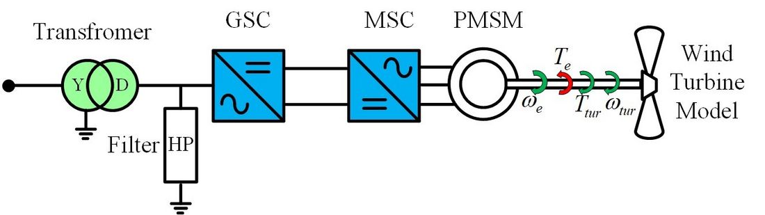
Figure 5 - Simplified circuit of wind energy system
The AC − DC − AC power electronic converter consists of a back-to-back two-level converter, providing full-scale power to the AC grid. The AC grid-side converter is known as a grid-side converter (GSC) and controls the back-to-back two-level converter’s DC-link voltage and AC/reactive power support. Due to the two-level converter, the converter is accompanied by a high pass (HP) filter to filter out higher frequencies. The machine-side converter (MSC) connects PMSM to the back-to-back two-level converter’s DC link. This converter acts as a variable-frequency VSC system. The MSC controls the stator voltage and PMSM torque. The detailed parameter calculation procedure of the GSC and MSC reader can be found in [19] and summarised in Tables V and VI. The control architecture of GSC and MSC will be explained in the following section. A scaling transformer is used to model the wind power plant, which acts as an interface between the lower-power wind turbine and the offshore converter station.
The wind speed data is uploaded to RSCAD®/RTDS via co-simulation. The TCP/IP protocol connects RSCAD®/RTDS to the Python script. In this script, live wind data is collected every second from two locations (i.e., Orkney and Shetland regions) in the north sea via a website and then communicated to the wind speed slider in RSCAD®/RTDS via TCP/IP protocol.
| Parameter | Values |
|---|---|
Rated generator power, GR | 2.5 MVA |
Rated turbine power, TR | 2.5 MW |
Generator speed (pu) at rated turbine speed, WR | 1.0 pu |
Rated wind speed, WSR | 12.0 m/s |
Cut-in wind speed, WSCI | 6.0 m/s |
Power coefficient type | ONE |
coefficient, | 1.0 |
Maximum wind speed, Vwpu,max | 1.5 pu (i.e., 18.0 m/s) |
Maximum power, Pturpu,overload | 1.28 pu |
Kp | 200.0 |
βmax | 36◦ |
| Parameter | Values | Parameter | Values |
|---|---|---|---|
Line-line root-mean-square (RMS) voltage, VLL,rms | 35 kV | Rated winding voltage at the converter side, VtrCon | 0.69 kV |
fundamental frequency, fo | 50 Hz | Transformer capacity, Str | 2.5 MVA |
Real power delivered to the point-of-common-coupling (PCC), Ps | 2.5 MW | Per-unit leakage inductance, Xtrpu | 0.1 pu |
Switching frequency of the converter, fsw | 2.0 kHz | Inductance of filter, Lf | 0.12 mH |
Dc-link voltage of the converter, Vdc | 1.2 kV | Capacitance of filter, Cf | 500.0µF |
System efficiency, η | 96% | Resonant Frequency, fres | 10fo< 649.7 Hz <fsw/2 |
Power factor at the PCC, pf | 1.0 | Damping Resistor, Rf | 0.122 ohm |
|
| Dc-link capacitor, Cbus | 70000.0 µF |
3. Control and protection overview
The onshore converter station (CSA1) regulates the DC voltage and acts as a slack bus. At the same time, rest converters are set into P-Q mode. The offshore converters are grid forming, i.e., the V-f control model. The internal protection of converter stations is enabled during the network energizing. The wind turbine act as a grid following converters. Thus inject the rated power at the rated wind speed. All the controls are realized by using a PI controller.
3.1.Control system in converter station
The control hierarchy of the converter station is adopted from [20] and summarised in this section. In the MTDC, each onshore converter station consists of three primary control loops [20], namely, outer voltage control (OVC), inner current control (ICC), and circulating current suppression control (CCSC), as shown in Figure 6. Figure 6 highlights the PI controls of the onshore and offshore converters. The OVC provides references to the ICC. The dispatch level provides the setpoints to the OVC via TCP/IP communication interface. The setpoint signals include a DC voltage Vdc,ref, an AC voltage Vac,ref, an active power Pac,ref , and a reactive power Qac,ref, and frequency f. The selection of these signals depends upon the control mode (i.e., constant DC voltage, grid forming/Islanded mode, active-reactive power control mode). The system operators/DC grid controller typically operate the dispatch controls. The system operators/DC grid controller provide the setpoint based on AC/DC power flow and day-ahead demand. Furthermore, a negative sequence control option is also introduced in the ICC, as shown in Figure 6(b).
The ICC loop generates the modulating voltages () based on the feedforward terms (
and
). In the case of sequence control, a double synchronous reference frame (DSRF) is used to express voltage and current into a positive (+) and a negative (−) sequence component. Furthermore, to eliminate the
frequency component in the DC current and voltage, the reference to the negative current sequence component (
) is set to zero, as shown in Figure 6(b). However, according to the ENTSO-E grid codes for specific nations [21], this control might have practical implementation restrictions.
The ICC and OVC are only responsible for the AC grid current's fundamental and odd-harmonic components. The CSCC controls the DC and the even harmonic components of the AC grid current, whose presence is responsible for the generated losses in the converter. Hence, these currents are suppressed by generating modulated voltage (), and as a result, only the DC component is present.
The islanded mode is realized by enabling direct voltage control (DVC) is enabled, which is the simplest form of grid-forming control [20]. Likewise, onshore converters, the offshore converter during the islanded mode of operation, receives setpoint commands from the dispatch control. Generated modulated voltages () are then applied to the lower-level control (LLC), which comprises dq−abc transformation and sort-and-select submodule modulation. Traditionally, these controls are implemented by applying PI controllers to transform AC measurements from the abc-frame into the stationary dq-frame using a phase-locked loop (PLL), except for a grid-forming control using an oscillator [1].
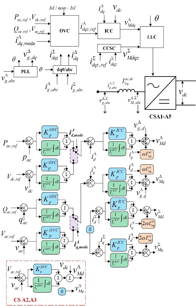
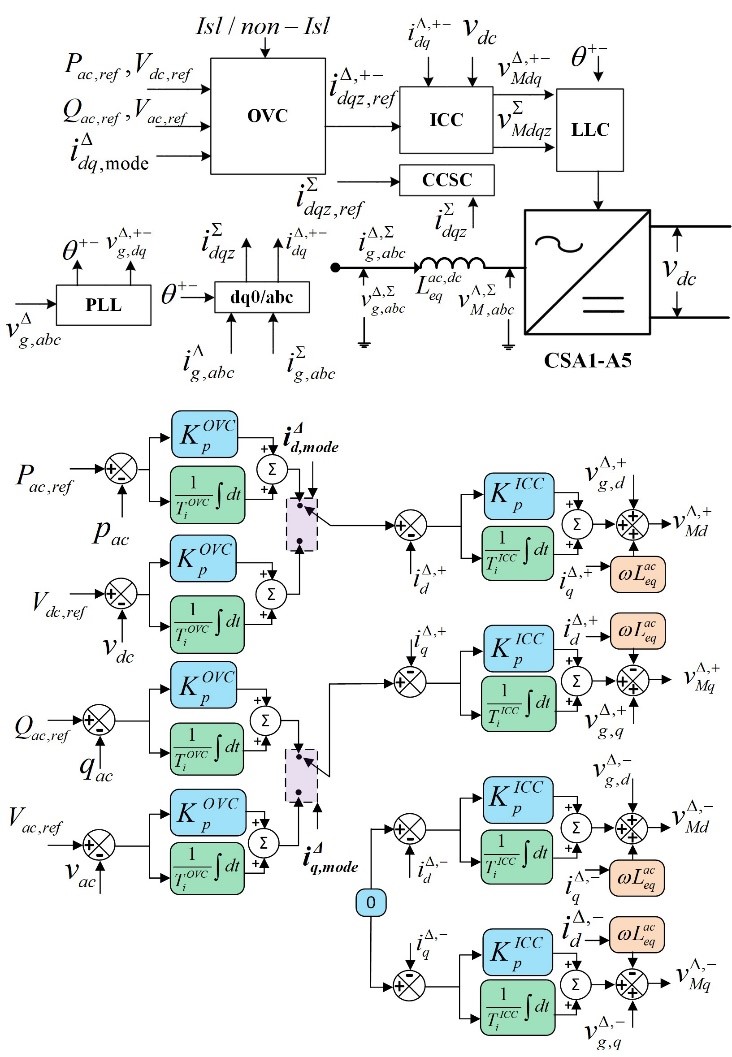
Figure 6 - Different Control strategies : (a) Traditional PI-based control ; (b) Sequence PI-based control
3.2. Control System in Wind Turbine
The control system of the type-4 wind turbines is the same as reported in [19] and [22]. To enhance the readability, the control system is summarised in this section. As explained in the previous section, type-4 wind turbines consist of two back-to-back full-scale converters.
Each converter possesses a specific control objective. The OVC loop provides the current references to the ICC loop, as shown in Figure 7. The GSC control controls the DC link voltage (Vdc) through the direct current component, while the quadrature component of the current controls reactive (or AC grid side voltage). Similar control loops can be seen in the MSC. However, the control objective for the MSC is different. In this work, the direct current of the converter regulates the stator terminal voltage. The stator voltage set point is kept at the rated voltage. The quadrature current of the converter controls the torque. The torque reference is given by , where
is the optimal coefficient of the maximum attainable turbine power and Wr is the wind turbine rotor speed.
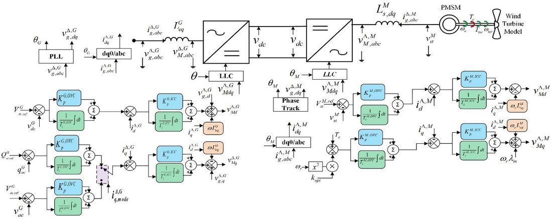
Figure 7 - Control loops in wind turbine
3.3. Converter protection and DC CB
During the transient event, protection is essential for component and system safety. The converter is protected from overcurrent during unscheduled events. This work considers full selective Fault Clearing with a DC CB protection scheme [23]. This scheme uses fault current limiters and DC CB to clear the fault. The primary purpose of this scheme is to keep the grid operating during the DC fault. The protection algorithm blocks the converter when the converter arm currents exceed the threshold value. The IGBT rating determines this value. It is set to be two times the rated current through the IGBT in this work.
Furthermore, the overcurrent protection is not triggered during the energization. The overcurrent protection of the converter also considers an overcurrent period. This protection is in an inactive state for a dormant period. The dormant period is determined by the operating time required by the DC CB to operate. Since VARC DC CB is employed, this dormant period is set to 5 ms. To avoid any complexity, the detection algorithm of DC CB is based on the rate of rise of the fault current. If the rate is above 4 kA/ms, the trip signal is provided to the DC CBs. Upon receiving a trip command, the breaker operates and interrupts the fault.
4. Computation load and core assignment
RSCAD®/RTDS make use of different core-based simulation environment, namely, Mainstep, Substep, Small Time-step, and Super step. Since power electronic-based devices operate in high-frequency bandwidth (<3kHz), the required time-step is in the range of 1.4μs– 3.75μs.
Considering this requirement, power electronic-based devices can be modeled in Substep or Small Time-step simulation environment. The substep simulation environment is state-of-the-art since it does not have a transmission line interface. As a result, artificial losses are exempted at high frequencies, as seen in a Small Time-step simulation environment. However, the disadvantage of the Substep simulation environment is that it takes up the entire Core and needs new NovaCor®. To make the model backward compatible (.i.e, older processors), optimal core utility, and lower switching frequency of MMC, a Small Time-step simulation environment is chosen in this work for modeling MMC. However, users are free to convert the same network to a substep simulation environment with the conversion tool provided by RSCAD® suit.
Depending on the network, the core and time steps are shown in Figure 8. The offshore converters are placed on a single core in all networks, as shown in Figure 8(b). In the case of the 5-terminal network, the minimum number of required cores is 7. These cores’ distribution can be down based on the simulation environment and element modeled. The converter station is modeled in a small-time step environment. Each onshore converter station requires a dedicated core, whereas the offshore converter stations run on a single core. The main reason for this is to reduce the core requirement. However, placing offshore converters on a single core increases the computation time. Hence, the requested time step for the Small Time-step environment consisting of an offshore converter is 2.8 µs. In contrast, the time step for a Small Time-step environment consisting of an onshore converter is set to 2 µs. The type 4 wind turbines, cables, and control system run in the main time step. Due to the large control signals and measurement, the main time step is about 60 µs.
Figure 8 (a) non-integer core values show the calculated Core required based on the processor assignment tab in RSCAD. For example, a maximum of 300 load units is fitted in one Core. However, for 5 terminal networks, the Network solution needs 420 (1.4 core) load units. Other main step elements require 470 load units (1.5 cores). These two can share cores, unlike a small time-step simulation environment. Thus total will be 2.9 cores. In reality, the Core is an integer. Thus closest maximum value will be 3.
In the four-terminal network, the onshore converters are placed on a single core, as seen in Figure 8(a); as a result, the time-step requirement is higher than in other networks. Thus, 2.75 µs is chosen for a small-time step environment. The main simulation time is set to 55 µs as the power and control load is reduced. Since the number of converter stations, cables, and control components is reduced for 4, 3, and 2 terminals networks, the net minimum requirement of the cores is 4, 4, and 3, respectively. With a lower computation load, the main time step of the network is lower for 3 and 2-terminals.
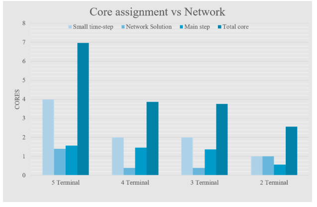
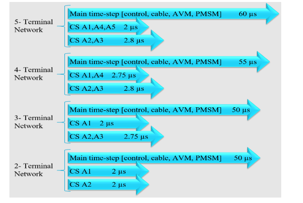
Figure 8 - For different networks : (a) Core assignment ; (b) Time-step assignment
5. Network Features
The network proposed in this work consists of the following feature:
- Aggregated Wind Turbines model: The model uses an Average value model of the converter to represent the wind farm without losing the dynamics of wind turbines. The Aggregation of a wind turbine is done by a scale transformer, where a factor amplifies the current. This avoids high computation load.
- Scripted Parameter: The important physical and control parameters are controlled by a script, reducing modeling time. The script controls the draft variables in RTS’s human-machine interface (HMI).
- Average Model of VARC DC CB: The Average employed model of DC CB uses passive and non-linear elements, reducing the computation load without losing the critical feature of breakers.
- DMR cable model: Both land and sea cables are modeled using Frequency Dependent (Phase) model with data based on the experience of 2GW Offshore Interconnection projects in the North Sea. This accurately models the dynamic metallic return (DMR) cables.
- Negative Sequence control: To have the minimum impact of AC imbalances, a negative sequence in an onshore converter is introduced in this work.
- Starting sequence: The network includes a sequence of DC grid energization. This sequence is written in a script, making the energization process flexible for the user
- Modular modeling: The networks enable easy replicability of the converter stations. Hence, the DC grid can be expanded based on user requirements.
- Converter Protection: The network provides a converter overcurrent protection, as explained in the previous section
- Real-time wind profile: The network captures wind speed data in real-time from a location in the north-sea using a SiL setup. The wind data is updated every 100 ms.
- Different control modes: This network also comprises different control modes presented in CIGRE 604 [20].
6. Simulation results
This section investigates unscheduled events and startup and black start sequences for the five-terminal network. Similarly, different steady-state and transient studies can be performed for the selected networks and are omitted in this work due to page limitations. However, these studies are highlighted in the next section.
6.1. Unscheduled Events
In the unscheduled events, three scenarios are considered. Namely, Single phase to ground (SLG) fault on the offshore AC side, Positive pole to ground (PG) fault on the DC side, and SLG fault on the onshore AC side. A temporary SLG fault of 200 ms in the offshore AC grid near CSA2 causes a drop in the AC voltage at PCC, as seen in Figure 9 (I-d). This fault causes a decrease in power and second-order fundamental frequency oscillation (figure 9 (I-c)). Further, this oscillation is propagated into the DC grid through DC link voltage and converter current, as shown in Figure 9 (I-a and I-b), which impacts AC grids connected to DC grids. Similarly, the network is tested for a PG fault near the terminal of CSA1, and the simulation results are presented in Figure 9 (II).
During the fault, net DC-link voltage reduces, as seen in Figure 9 (II-a); however, it is interesting that even at fault near the CSA1 terminal, DC-link voltage at the CSA2 terminal reduces. This is due to the uncontrolled power dispatch during the fault between the DC cables. The DC CB completely interrupts the fault current 5 ms. Once the fault current interrupters, the DC fault current stops rising due to high impedance by the surge arrester of DC CB. Since there is no increase in the fault current (i.e., after 5 ms of fault occurrence), the internal protection of MMC is not triggered. After the fault interruption, DC grid coverage to a new stable equilibrium point.
Figure 9.1(III) shows the impact of 200 ms SLG onshore fault near CSA1. The figure also compares AC faults with and without negative sequence control. As discussed in the previous section, the onshore converter stations are employed with negative sequence control; the presence of this control reduces the amplitude of the second-order fundamental frequency component, as seen in Figure 9 (III-b,d, and f) compared to the traditional control scheme. This second-order oscillation arises due to an imbalance in the AC voltage (figure 9 (III-g)). Thus by controlling the positive sequence current component and setting the negative sequence current component to zero, the second-order of the fundamental frequency is regulated in the DC grid.
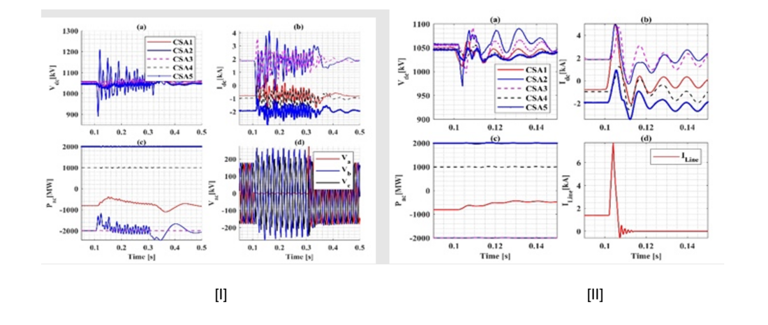
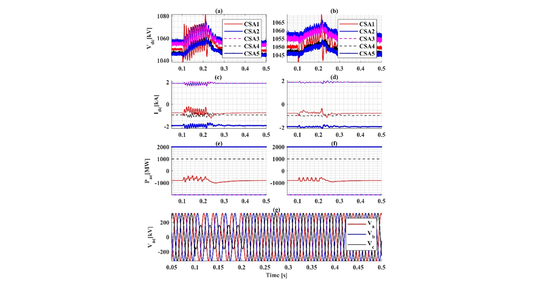
Figure 9 - [I] SLG fault on the offshore AC side, where (a) DC link voltage, (b) Positive pole DC of CS, (c) Active Power of CS, and (d) Three phase offshore voltage at PCC, [II] Positive pole to ground (PG) fault on DC side, where (a) DC link voltage, (b) Positive pole DC of CS, (c) Active Power of CS and (d) Positive pole DC through cable 1 and [III] SLG fault on the onshore AC side, where (a),(c) and (e) are DC link voltage, Positive pole DC of CS and Ac-tive Power of CS without negative sequence control. (b),(d) and (f) are DC link voltage, Posi-tive pole DC of CS, and Active Power of CS with negative sequence control. (g) The three-phase onshore voltage at PCC.
With a temporary 3-phase fault to the ground at offshore converter (CSA2), active power injected by wind farms reduces significantly, as seen below in Figure 10 I-(c). The CSA1 partially compensates for this loss of power during fault. Rest power is drawn from the DC link causing a drop in the DC link voltage.
With a temporary 3-phase fault to ground at the onshore converter (CSA1), active power injected by wind power plants remains the same; however, due to fault near the converter controlling DC link voltage causes overvoltage due to the excess power in the DC-link for both type of controls (i.e., traditional and sequence control) as seen in figure 10 II-(a) and (b).
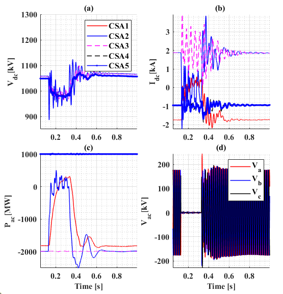
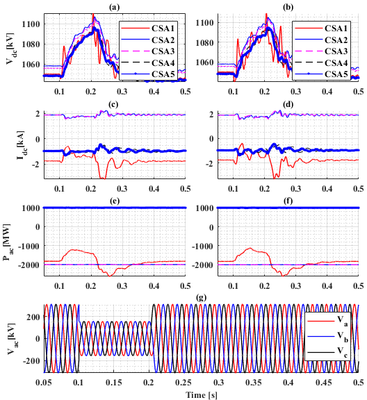
Figure 10 - [I] Three phase fault on the offshore AC side, where (a) DC link voltage, (b) Pos-itive pole DC of CS, (c) Active Power of CS, and (d) Three phase offshore voltage at PCC and [II] Three phase fault on the onshore AC side, where (a),(c) and (e) are DC link volt-age, Positive pole DC of CS and Active Power of CS without negative sequence control. (b),(d) and (f) are DC link voltage, Positive pole DC of CS, and Active Power of CS with negative sequence control. (g) The three-phase onshore voltage at PCC
These extreme events were performed to test the network's response. However, these are simulated scenarios, and the occurrence of fault during full load capacity is extreme. However, performing such studies aims to get an overall picture of the transient overvoltage and overcurrent profile, which will help design and specify the protection equipment’s setting and control strategies.
6.2. Startup and black start sequence
Table VII highlights different events carried out during the energization and black start of the five-terminal networks. Figure 11 illustrates the pole-to-pole voltage of five converter stations during the startup. This figure is only high transient due to events being labeled via numerical value. The description of these labels is indicated in Table VII.
At the start of simulations, all the converters and cables are de-energized. Hence, the energization occurs by first connecting the converter responsible for regulating DC-link voltage, i.e., CSA1. However, first, the pre-insertion resistance is connected to limit the inrush current. Since each converter station has two poles, a sequential connection of pre-insertion resistance is made. Firstly, the positive pole (CSA1P) pre-insertion resistance is connected, followed by the negative pole (CSA1N) pre-insertion resistance. This leads to the charging of the SM in the positive and negative poles. Once the converters are charged, the next step is to collectively charge the DC cables, considering using a disconnector and pre-insertion resistance. With the close of the disconnector, an extensive DC voltage transient, with a lower peak of -203 kV, is observed. Pre-insertion resistance is bypassed upon charging the DC cable to eliminate the loss during the steady-state operation. Similarly, a local impact of DC voltage at CSA2 and CSA3 is observed during the close of disconnectors at CSA2 and CSA3. Like CSA1, the CSA4 converter station is energized and connected to the DC grid.
Firstly, the DC voltage setpoint is kept at 80% of the rated DC voltage, and the converter CSA1 is deblocked. Since there is no offshore grid, CSA2 and CSA3 are deblocked, which creates a transient in the DC voltage, as shown in the zoom plot. Once the offshore voltage is stabilized, the collective black start of the wind farm is carried out. Followed by this event, the DC voltage is ramped to the rated voltage by changing the setpoints. As soon as the rated DC grid voltage is stabilized, 1 GW of each power into the DC grid by wind farm 1 and wind farm 2. After deblocking of converter CSA4, power is ramped to 1 GW into the onshore AC grid.
In this work, an investigation of new HVDC connections is also considered. This new connection is converter CSA5. Considering the stable operation, how the new connection impacts the stability and stress in the DC grid can be investigated. The impact is lower if the new converter station is precharged via the onshore AC grid. However, a sharp transient is observed in the pole-to-pole voltage of converter CSA5 upon re-closing the disconnector. Furthermore, the power setpoint of CSA5 creates an overload in the network, especially in the DC cables and CSA1.
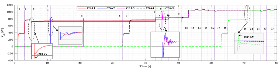
Figure 11 - Pole-to-pole voltage of different converter stations during startup
| Events | Time (sec) | Events | Time (sec) |
|---|---|---|---|
Enable pre-insertion resistance at CSA1P (1) | 1 | Changing the DC link voltage setpoint to 0.8 pu | 41 |
Enable pre-insertion resistance at CSA1N (2) | 3 | Deblock CSA1 (8) | 43 |
Close the DC grid disconnector at CSA1 (3) | 5 | Deblock CSA2 (9) | 45 |
Bypass pre-insertion resistance at CSA1P | 7 | Close the DC grid disconnector at CSA4 (10) | 47 |
Bypass pre-insertion resistance at CSA1N | 9 | Deblock both the wind farm | 49 |
Close the DC grid disconnector at CSA2 (4) | 11 | Deblock CSA3 (11) | 51 |
Enable pre-insertion resistance at CSA2P | 13 | Changing the DC link voltage setpoint to 1 pu (12) | 53 |
Enable pre-insertion resistance at CSA2N | 15 | Increasing wind power to 1GW at WF1 (13) | 55 |
Bypass pre-insertion resistance at CSA2P | 17 | Increasing wind power to 1GW at WF2 (14) | 57 |
Bypass pre-insertion resistance at CSA2N | 19 | Deblock CSA4 (15) | 59 |
Close the DC grid disconnector at CSA3 (5) | 21 | Changing the Active power setpoint to 1000 MW at CSA4 (16) | 61 |
Enable pre-insertion resistance at CSA3P | 23 | Enable pre-insertion resistance at CSA5P (17) | 63 |
Enable pre-insertion resistance at CSA3N | 25 | Enable pre-insertion resistance at CSA5N (18) | 65 |
Bypass pre-insertion resistance at CSA3P | 27 | Bypass pre-insertion resistance at CSA5P | 67 |
Bypass pre-insertion resistance at CSA3N | 29 | Bypass pre-insertion resistance at CSA5N | 69 |
Close Wind Farm disconnectors | 31 | Close the DC grid disconnector at CSA5 (19) | 71 |
Enable pre-insertion resistance at CSA4P (6) | 33 | Deblock CSA5 (20) | 73 |
Enable pre-insertion resistance at CSA4N (7) | 35 | Changing the Active power setpoint to 1000 MW at CSA5 (21) | 75 |
Bypass pre-insertion resistance at CSA4P | 37 | Increasing wind power to 2GW at WF1 (22) | 77 |
Bypass pre-insertion resistance at CSA4N | 39 | Increasing wind power to 2GW at WF2 (23) | 79 |
7. Studies and analysis performed on the proposed network
Based on the guides provided in Cigre B4-832 [6], the proposed network can be used during different life cycle studies. During the project's preliminary phase, these networks can be used to determine the DC fault performance, impact of new HVDC link, preliminary DC cable investigation, grid code studies, AC system equivalent impact, and overvoltage investigations. In the bid phase, these networks can be used for measurement points, signal name determination, transient stress, and dynamic performance studies. During the implementation phase, the studies, as mentioned earlier, can be investigated in detail using these networks via analysis in Table VIII.
Transients Analysis during normal operation | Setpoint changes and load rejections |
Startup (energisation) sequence | |
DC system discharging | |
Switching operations | |
Black start – sequential and collective energisation. | |
Grid-side transients analysis | Grid side faults |
Switching operations and abnormal operating conditions | |
DC side transient analysis | DC side faults: Internal and external faults |
DC cable voltage stress: Impact of cable segments | |
Failure mode analysis of DC CB | |
Interaction studies | Parallel VSC-HVDC |
Offshore wind power plant | |
Interaction due to DC grid | |
Interaction between converters | |
Interaction due to non-linear function |
8. Conclusion
This paper has introduced real-time network models of a multi-terminal HVDC power system with real-time wind profile feedback., The models can be used for performing different life cycle studies of HVDC projects. The proposed network models address the shortcomings of existing network models in technical brochures and are designed for the system ratings required by the north-sea grid operator. The models provide accurate parameters for dedicated metallic return (DMR) sea and land cables, and the system and control parameters are scripted, reducing modeling time for perturbation and sensitivity studies. The proposed models also consider the average value model of wind farms, enabling investigation into the interaction and dynamics caused by wind farms.
The performance of the models is evaluated using unscheduled events, startup, and black start events, and it was observed that the presence of the frequency component was reduced during SLG fault at onshore PCC due to the implementation of negative sequence control. However, the SLG fault at offshore PCC caused large disturbances in the offshore grid, which were transmitted into the DC grid. Different stress points were observed in the startup and black start sequence, which will be crucial during component design and protection studies.
Additionally, the paper illustrated the computational requirement per network model, which will help users select the appropriate model depending on the modeling requirement. Finally, the paper discussed future studies that can be conducted using the proposed network, which will assist users in defining component design and system calculation. Overall, the proposed real-time network models with wind profile feedback provide a valuable tool for manufacturers and system operators to perform different life cycle studies of HVDC projects, ultimately contributing to the development of more efficient and reliable HVDC grid systems.
The network provides new voltage ratings and cable models for upcoming European projects and can be starting point for system studies and control system design. Furthermore, these networks can be used for training and developing a new set of skills the system operators need.
9. Appendix A. Screen-short of five-terminal HVDC network
Figures A.1 and A.2 show the runtime and dft file screenshots of the developed five-terminal HVDC network in RSCAD®/RTDS. In Runtime, the converter station, the DC grid, and the wind farm have been grouped so that users can easily change the layout or duplicate the elements. Each converter station has a draft parameters group, a control group, and measurements. Furthermore, the draft parameters are controlled by a script for automation purposes. The draft parameter includes electrical and control data. The control group consists of different modes of converter and setpoints. The color of the converter indicates the blocking state of the converter; the green color indicates the deblock state and the red color indicates the block state.
The DC grid comprises cable connections, a breaker state, and power measurements. The wind farm group comprises measurement and scaling factors. At the 815 value of the scaling factor, the power injection is 2 GW. The energization control of the wind farm is placed in the main canvas. The main canvas also includes the wind speed of both wind farms. The script controls this to improve the onsite live data in the RTS. Similarly, the push button triggers the onshore, offshore, and dc faults. Furthermore, it can be cleared/reset with the reset button.
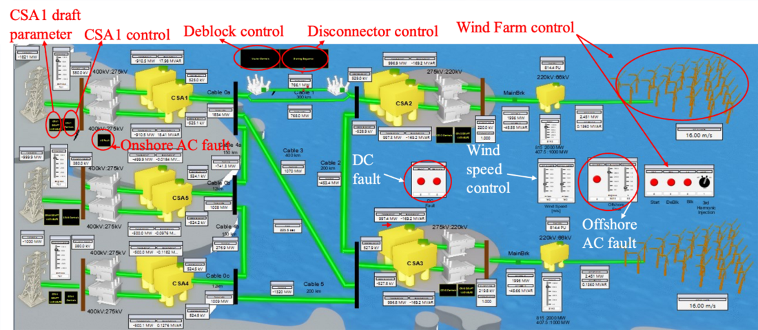
Figure A.1 - Steady state screenshot of 5-Terminal HVDC network
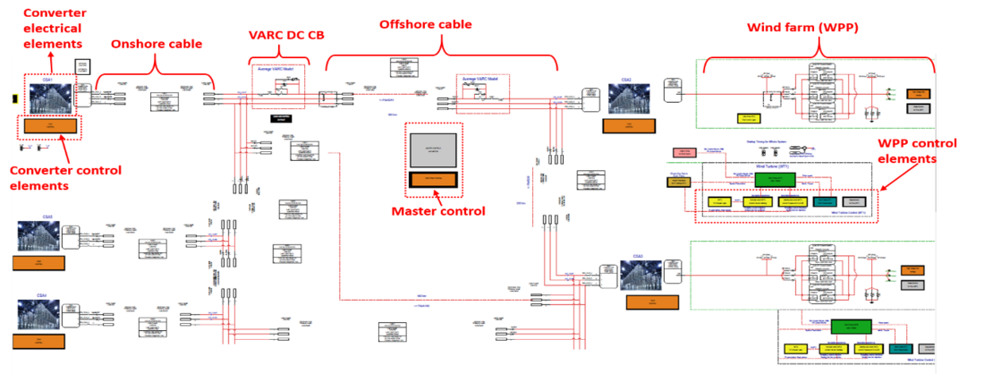
Figure A.2 - DFT file screenshot of 5-Terminal HVDC network
10. References
- CIGRE Working Group B4.72, “DC grid benchmark models for system studies,” CIGRE Technical Brochure, vol. 804, no. June, 2020.
- L. K. G. Chaffey, W. Leterme, D. Van Hertem, O. Adeuyi, I. Cowan, B. Ponnalagan, M. H. Rah-man, I. Jahn, K. Ishida-san, “D9 . 1 – Real-time models for benchmark DC grid systems,” 2020.
- M. Wang, W. Leterme, G. Chaffey, J. Beerten, and D. Van Hertem, “Multivendor interoperability in HVDC grid protection: State-of-the-art and challenges ahead,” IET Gener. Transm. Distrib., vol. 15, no. 15, pp. 2153–2175, 2021, doi: 10.1049/gtd2.12165.
- BESTPATHS, “BEST PATHS D9.3: Final Recommendations For Interoperability Interoperability of Multivendor HVDC Systems,” Tech. Rep. D9.3, vol. D9.3, pp. 1–73, 2018.
- CIGRE Working Group B4.74, “Guide to Develop Real-Time Simulation Models for HVDC Operational Studies,” CIGRE Technical Brochure, vol. 864, no. February, 2022.
- CIGRE Working Group B4.70, “Guide for electromagnetic transient studies involving VSC converters,” CIGRE Technical Brochure, vol. 832, no. April, 2021.
- CIGRE Working Group B4.76, “DC-DC converters in HVDC grids and for connections to HVDC systems,” CIGRE Technical Brochure, vol. 827, 2021.
- A. Shetgaonkar, A. Lekić, and M. Popov, “HVDC RTDS models,” Git hub, 2023. https://github.com/control-protection-grids-tudelft/HVDC-RTDS-models.
- CIGRE Working Group B4.57, “Guide for the Development of Models for HVDC Converters in a HVDC Grid,” CIGRE Technical Brochure, no. 604, 2014.
- Y. Murata et al., “Development of high voltage dc-Xlpe cable system,” SEI Tech. Rev., no. 76, pp. 55–62, 2013.
- A. Abbasi, A. Hoang, E. Eriksson, and F. Fälth, “Performance evaluation of 525 kV and 640 kV extruded DC cable systems,” in 10th International Conference on Insulated Power Cables, 2019, pp. A9-4.
- E. Commission,“REPowerEU: affordable, secure and sustainable energy for Europe.”, 2023.
- C. Electra, “ELECTRA N ° 321 April 2022,” no. April 2022, pp. 1–115, 2023.
- Federal Ministry for Economic Affairs and Energy, “Electricity 2030,” p. 52, 2017, [Online].
- S. Liu et al., “Modeling, Experimental Validation, and Application of VARC HVDC Circuit Breakers,” IEEE Trans. Power Deliv., vol. 35, no. 3, pp. 1515–1526, 2020, doi: 10.1109/TPWRD.2019.2947544.
- A. Shetgaonkar, S. Liu, and M. Popov, “Comparative Analysis of a Detailed and an Average VARC DCCB model in MTDC Systems,” in IEEE Power and Energy Society General Meeting, 2022, vol. 2022-July, doi: 10.1109/PESGM48719.2022.9916949.
- CIGRE Working Group B4.62 , “Connection of Wind Farms to Weak AC networks,” CIGRE Technical Brochure, vol. 671, 2016.
- T. Sebastian and G. R. Slemon, “Transient Modeling And Performance Of Variable-Speed Permanent-Magnet Motors,” IEEE Trans. Ind. Appl., vol. 25, no. 1, pp. 101–106, 1989, doi: 10.1109/28.18878.
- RTDS Technologies, “Standardization of Renewable Energy System Modelling,” 2022.
- CIGRE Working Group B4.57, “Guide for the Development of Models for HVDC Converters in a HVDC Grid, CIGRE Technical Brochure N.604, 2014.
- ENTSO-E, “Fault current contribution from PPMS & HVDC,” 2016.
- A. Shetgaonkar, A. Lekic´, L. Liu, M. Popov, and P. Palensky, “Model Predictive Control and Protection of Mmc-Based Mtdc Power Systems,” Int. J. Electr. Power Energy Syst., 2022, doi: 10.2139/ssrn.4127026.
- W. P. 4 Promot. Project, “Broad comparison of fault clearing strategies for DC grids,” 2022. [Online].
- [1] HVDC RTDS models : github.com/control-protection-grids-tudelft/HVDC-RTDS-models