Bayesian Risk-based Maintenance for High Voltage Assets: A practical approach
AUTHORS
H. SCHNITTKER, P. WERLE - Institute of Electric Power Systems, Division of High-Voltage Engineering and Asset Management - Schering-Institute, Leibniz University Hannover, Hannover, Germany
B. HELING - TenneT TSO GmbH, Bayreuth, Germany

Summary
Risk-based maintenance can help utilities overcome the challenges of the energy transition. However, assessing the risk of the assets is often difficult and needs to take into account the individual needs of the utility. This article describes a risk-based maintenance approach for high-voltage assets with a Bayesian view of probability. This allows a quantification of the failure probability, and therefore the risk, of each individual asset. The chosen interpretation of risk-based maintenance naturally includes existing maintenance strategies, which simplifies a practical implementation. Further, the approach is versatile through the possibility to use different kinds of available information, combining the information and varying the depth of the analysis by including failure modes. In this way, the individual needs of the utilities can be addressed.
Keywords
Asset management for utilities - risk-based maintenance - health index - Bayes' theorem - probability assessment1. Introduction
The increasing energy flows in the course of integrating renewable energies and their sector-coupled use require an expansion of the electricity grids [1] and put different, often higher stress on assets of the electricity grids [2]. At the same time, a considerable number of assets reach their scheduled end of life and must be renewed [3]. In addition, the European Union demands a risk assessment for all relevant risks relating to the security of electricity supply to assure reliability [4]. This task of assuring reliability becomes more challenging. Firstly, in the course of the energy transition, the surplus of the system capacity decreases and new mega assets like the Suedlink [5] with high impact on reliability supplement the system. Secondly, the demographic change and the accompanying shortage of specialists lead, together with the grid expansion, to an increasing number of assets to be managed per headcount [6]. Asset management (AM) can help overcome these challenges by translating "the organization’s objectives into asset-related decisions, plans, and activities, using a risk-based approach" [7]. In general, reliability depends on the system capacity, redundancy in the system, quality of the components and assemblies, design safety factors, surveillance in operation, and maintenance activities.
With the focus on maintenance, utilities often use their own, self-developed health index approaches to increase their reliability with a trend toward risk assessment (cf. section 2.1). A central difficulty of risk-based maintenance is quantifying the risk and especially probability of that risk. Here, Bayesian inference has attracted significant attention, and sophisticated Bayesian networks have been developed (cf. section 2.2). However, the practical application among utilities is rare because these models are often unsuitable for direct implementation. Utilities usually lack requirements like complete analyses or data for an application of Bayesian networks (cf. section 2.2).
The novelty of the presented work lies in a new combination that links the existing maintenance of utilities, risk-based maintenance, and Bayesian inference. Therefore, a basic risk model is proposed, which allows individually quantifying the probability of failure with the data available. So, the particular characteristics of utilities and high-voltage assets are regarded. This procedure can be used directly as a low-level approach to facilitate the implementation of risk-based maintenance. In this way, the basic structures can be established on which advanced assessments can be built.
The text is organised as follows: section 2 recapitulates important aspects of risk-based maintenance and health-index procedures, as well as Bayesian statistics. In section 3, the basic model is introduced. Then the versatility is shown by including failure modes for a detailed assessment, and combining different information. Finally, in section 4, the model is demonstrated on an example of a circuit breaker.
2. State of the Art
2.1. Risk-based Maintenance and Health Index
There are two significant aspects in maintenance: firstly, identifying the need for a maintenance measure (trigger) and secondly, determining an order and/or bundling of measures (prioritisation) [8]. Theoretically, both aspects are based on a necessity to save or a possibility to increase value, which clarifies the connection to AM, since it is defined as the "coordinated activity of an organisation to realise value from assets" [7]. A possibility to increase value can be a maintenance measure to prolong the lifetime of an asset, or using a renewal of a street to lay a cable to save earthwork costs. A necessity to save value can be a restriction or limitation such as imminent failures, legal requirements, budget, deadlines, switching approvals, human resources, delivery times, etc. The various maintenance strategies address triggering and prioritisation differently: Corrective maintenance (CM) initiates a maintenance measure after a failure, thus CM can be used to trigger maintenance measures [9],[10]. Time-based maintenance (TBM) carries out maintenance measures in regular intervals based on periods, which often is a time interval but can also be operational parameters [9],[10]. The interval triggers the measures, and by varying the interval a kind of prioritisation is possible. Condition-based maintenance (CBM) triggers a maintenance measure dependent on the condition [9],[10]. The condition also enables prioritising measures. Naturally, the asset with the worst condition has first priority, which is not always the best choice since the consequences of a failure are not considered. Reliability-centered maintenance (RCM) puts the consequences in the foreground – not the avoidance of a failure per se [11]. The Failure Mode Effects Analysis (FMEA) developed in this context systematically analyses failure causes and defines failure modes. Often, the effects of a failure are determined by the severity and are commonly distinguished into major failure (MaF) and minor failure (MiF). MaF lead to a non-functionality of the system, while with a MiF the system is able to fulfil its basic functions [11],[12]. Assessing the consequences can be used to prioritise the maintenance measures, but it is less suitable for triggering. Risk-based maintenance (RBM) enables calculating the risk of a failure as in (1) [13],[14].
(1)
The risk triggers a maintenance measure when exceeding the threshold of a risk value. This will be the case if the probability or the consequences changes. After a risk assessment, the measures are prioritised. A possible example is an order which first addresses the measures reducing the highest risk, or an order which first addresses the measures with the highest risk mitigation. It should be emphasised that consequences can be positive, resulting in a positive risk or chance. Mitigating risk or using a chance is comparable to increasing value in AM. Therefore, a risk-based approach is able to model the basic AM idea.
In practice, utilities often use health index procedures for condition assessment [15]. These procedures are heterogeneous and not clearly defined since each utility sets its own priorities and has developed its own procedure and best practice method on the basis of the internal and external environment that confronts it. Generally, the health index procedures share the commonality of assigning an index number on a scale (e.g. 1-10 or 1-100) to each asset. In addition, a categorisation (e.g. good, moderate, and poor) in combination with a colour code (e.g. green, yellow, and red) is often used for ease of reference. A health index thus creates an order whose elements up to a threshold value cause actions to be triggered. The order can also be used directly for prioritising measures. Depending on whether the focus of the health index is on triggering or prioritisation, the number has a different meaning. Most of the time, this number reflects a condition or failure probability of an asset, but also an order of repair measures is possible. CIGRE WG A2.49 thus recommends an earmarked health index to emphasise the intention, e.g. reliability index or repair index [16]. There are sophisticated health indices using a risk-based approach (e.g. the CNAIM model [17]), which fits well with the theory above. This view of a health index is as well supported by CIGRE's TB 858 [18] and Jasni et. al. [19]. Also, in other infrastructure systems like railway systems, risk-based approaches are used [20].
Currently, asset management of utilities is dominated by a time-based trigger for maintenance measures and a condition-based trigger for replacements with no prioritisation [15]. When switching to RBM, utilities have to mind that there is no unique way to perform risk analysis and risk-based maintenance [21]. ISO 31010 lists 31 tools and techniques for risk identification, risk analysis, and risk evaluation with individual advantages and disadvantages [22]. Therefore, every utility has to choose its own appropriate solution, which will be an ongoing process. Following this argumentation, it is convenient to implement RBM without a complete reorganisation of maintenance. Thus, the proposed and used interpretation of RBM is that it already includes the other maintenance strategies (cf. Figure 1). So, if a failure occurs before the threshold value is reached, RBM can be seen as CM. If an increase in probability is assumed over time, RBM is based on TBM. If the probability is assessed, it can be interpreted that RBM is based on CBM, or if the consequences are assessed systematically, RBM can be seen as based on RCM. This interpretation has the advantage that utilities can retain pre-existing maintenance procedures, and implement RBM stepwise in dependence on available data, the needs of the utility, and cost-benefit consideration, thus providing the necessary versatility.

Figure 1 – Underlying interpretation of the maintenance strategies
2.2. Bayesian Statistic
In maintenance, especially for high-voltage assets, it is often valid that the sample size is small, the failure rate is low, the lifespan of the assets is long, and maintenance measures include a large share of expert know-how. The Bayesian view of inference allows convenient interpretation of the findings and consequently forms the basis for the developed maintenance model. The central element of the model is Bayes’ theorem (5).
(5)
As detailed below, the a priori probability p(X) is updated by a factor to obtain the a posteriori probability p(X│Y).
The inferential statistic describes inferences from a sample of a larger population. There are two prevailing views: the classical or frequentist statistic and the Bayesian statistic. The classical statistic defines probability as the relative frequency in random experiments. Therefore, only the sample is used to estimate parameters or to test hypotheses. The Bayesian statistic defines probability as an expression of knowledge, thus further assumptions or knowledge of a problem are possible to consider [23]. Both views use the same calculation rules, which are based on the three axioms of Kolmogorov [24]. The axioms can be specified by two random variables X and Y.
X can take the values xi, with i = 1,...,M, and Y can take the values yj, with j = 1,...,L. Sampling X and Y in a total of N trials gives the number nij for X=xi and Y=yj. Further, taking xi and all yj is denoted by ci and taking yj and all xi is denoted by rj (cf. Figure 2.).
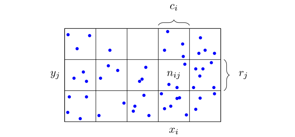
Figure 2 - Probabilities of the two random variables X and Y with M=5 and L=3 [25]
The joint probability for X = xi and Y = yj is given by the number of points falling in the cell i, j [24].
(6)
The conditional probability X = xi given Y = yj is obtained by the fraction of points in row j falling in the cell i, j [24].
(7)
Marginalizing X leads to the marginal probability of p( Y = yi ) (cf. (8)), which is the sum of the points in row j and is therefore referred to as the sum rule in probability. Marginalizing Y leads to the marginal probability of p(X = xi ) (9) [25].
(8)
(9)
The joint probability from (6) can also be expressed by the conditional probability (cf. (7)) multiplied by the marginal probability of (8), which is stated as the product rule in probability [25].
(10)
p(X = xi ) and ( Y = yi ) will be written in the more compact notation p(X) and p(Y). Then Bayes' theorem can be obtained using the product rule and the symmetry property p(X,Y)=p(Y,X) [25].
(11)
The second notation of (11) emphasises the interpretation of updating the a priori probability p(X) by a factor to get the a posteriori probability . The factor is not a probability and can be greater than 1, which increases the probabilityX, equal to 1, which does not change the probability, or smaller than 1, which decreases the probability.
Expanding the example by a third random variable Z provides (12) [23].
(12)
If the variables are independent, the equation simplifies to (13). In this way, every new variable creates a new factor, which updates the a priori probability [23].
(13)
The Bayesian view sees probability as an expression for a degree of knowledge, stated in the fundamental idea of updating a probability using Bayes' theorem, which enables assessing the probability of risk individually and versatilely. Therefore, utilities can use the information available for individual asset decisions.
Bayesian risk-based maintenance techniques are widely adopted in the maintenance of mechanical systems and in diagnosing deterioration. Here, Bayesian networks are the most common models connecting Bayesian inference and risk-based maintenance. These graphical models use directed graphs to describe probability distributions through nodes and edges [25], allowing for the analysis of dependencies, risks, and maintenance [26]. The oil and gas industry has shown significant interest in Bayesian networks, e.g. in natural gas reduction and measuring stations [27], as well as offshore applications, such as pipelines [28] or the safety of people onboard ships [29]. Also, other infrastructure systems like power plants [30] or railway systems [31] use Bayesian networks. Moreover, Bayesian networks are able to model deterioration processes [32]. However, a Bayesian network can only reach its full potential when maintenance is considered holistically. All factors of the to-be-maintained system and relationships between systems should be addressed [26]. But, utilities usually have incomplete analyses or data. Thus, utilities often miss the base for an application of Bayesian networks. Other risk assessments using Bayesian approaches, which are not based on Bayesian networks, are less popular. Apeland has developed two probabilistic frameworks that use Bayesian approaches to optimise risk analysis by describing an analyst group's uncertainty/knowledge [33]. Khan updates the gamma distribution of the average degradation rate of process plants by actual inspection results [34]. But, a profound database is also necessary to create the needed distributions.
Further approaches deal mainly with specific maintenance applications using Bayes’ theorem. For instance, Muratović has used Bayes' theorem to determine the failure distribution of a newly developed circuit breaker by combining historical failure data and information on failures during mechanical development tests [35]. Sørensen introduces a cost-benefit model for optimal inspection planning of offshore wind turbines based on Bayesian decision theory [36]. Dirbaz has also used Bayes' theorem to update discrete condition ratings of bridges through a visual inspection [37], which is similar to rudimentary health indices. In addition, Shindo has evaluated diagnostic results of deteriorated facilities more accurately [38], while Kallen has determined optimal inspection plans by updating a prior density distribution with an inspection measurement under uncertain deterioration [39]. Although these applications demonstrate the versatility of Bayes’ theorem, they do not offer a broadly applicable framework to help utilities with their different needs.
In summary, the challenges of the utilities lead to a trend towards risk-based maintenance. An interpretation of RBM, including other maintenance strategies, creates the versatility needed by the individual utility to implement RBM while being able to use pre-existing maintenance procedures. But especially for high-voltage assets, the probability involved in the risk evaluation is difficult to obtain. Here, Bayesian inference allows a convenient view of probability, where Bayes’ theorem updates probability with newly available knowledge. Bayesian networks seem promising, but the basic structures are missing for an application. Combining these points led to a Bayesian risk-based maintenance model for high-voltage assets, which is presented in the following.
3. Bayesian risk-based maintenance model
A basic model is proposed, which can be flexibly expanded and modified by including failure modes and functional units, or combing (different) evidence.
3.1. Basic model
The basic maintenance model describes the risk r of an asset through the probability and the consequences of an asset failure. In its simplest form, the probability is the failure rate λ and the consequences are the replacement costs c. Then, the probability of the asset failure is combined with the evidence indicating the failure. Therefore, the hypothesis is made whether there is a failure of the asset H or not ¬ H. Further, the evidence either indicating the failure E or not indicating the failure ¬ E is considered. Next, the conditional probability can be calculated using Bayes' theorem. Testing a hypothesis in Bayesian inference calculates the probability of the hypothesis, thus there are no null hypothesis, no significance level, and no accepting or refusing of the hypothesis [23]. The value of this approach unfolds in the two advantages of supporting objective decision-making and the versatility in combining evidence.
Objective decision-making is supported by a direct, reasonable linking of evidence to the condition. Generally, it is human to neglect the population and therefore overestimate the evidence [40]. Asset Managers try to avoid this overestimation by not trusting one sole evidence like a measurement which indicates a failure. Instead, a second measurement or different measurement will be performed to obtain evidence. Updating a prior probability using Bayes' theorem enables a quantity measure to make a more objective decision.
The following fictional example of an asset failure probability illustrates the procedure. The annual failure rate of this asset model is λ=1 %, and the replacement costs are c=10 000 €. The resulting risk r is calculated in (14).
(14)
Further, it is assumed that a measurement A detects a failure of the asset by a chance of 80% (e.g. a contact resistance measurement may not detect failures of the insulation system). Moreover, measurement A may wrongly sign a failure when there is no failure by a chance of 3 % (e.g. incorrect execution of the measurement). Then the hypothesis "failure of the asset" can be proposed and be connected to the evidence "measurement A" with the following probabilities:
- The a priori probability that the hypothesis "failure of the asset" is true is described by p(H)=1% as the annual failure rate of the asset.
- The probability that the hypothesis "failure of the asset" is false is described by p(¬ H), which can be obtained by
.
- The total probability of seeing the evidence is described by p(E). The blue-filled squares in Figure 2 represented this probability. Since p(E) is difficult to determine, it is often calculated by
.
- The probability that the evidence supports the hypothesis when the hypothesis is true is described by
as the chance of detecting the failure when there is an actual failure.
- The probability that the evidence supports the hypothesis even so the hypothesis is false is described by
as the probability that the measurement indicates a failure when there is no failure.

Figure 3 - The probability of the two random variables H and E [41]
Then Bayes' theorem is used to calculate the probability that the hypothesis is true after seeing the evidence .
(15)
The updated risk is thus 2120 € (cf. (16)).
(16)
In this case, measurement A updates the probability of a possible failure of the asset, which lead to a new risk. The adjusted risk may trigger a maintenance measure if a threshold is exceeded. Generalised, after obtaining new evidence about a circumstance, the knowledge of this circumstance is modified. The a priori probability p(H) updated by Bayes’ theorem is the a posteriori probability , which expresses a quantified degree of belief and thus supports an objective decision. It should be emphasised that the procedure aims for preventive maintenance. Many measurements give a sure output, e.g. measuring an open circuit or visually seeing an oil leakage. The probability of this evidence would be 100 %, which demonstrates the applicability, except the added value arises first from evidence, which not certainly shows a failure state but indicates an imminent failure. Often evidence with thresholds falls in this category. The threshold value marks an anchor point, whereas the decision-making is based on a range of values. E.g. if a contact resistance above 40
is considered a bad condition, it does not mean a failure will occur instantly after exceeding the value of 40
. Instead, the probability of a failure is considered high enough to initiate a measure. But in most terms, a value of 39
will also be a cause of concern.
For a practical application, two things are important: to be more selective or detailed in the diagnostic for one asset and to implement various, non-certain evidence.
3.2. Including Failure Modes and Functional Units
A more complex condition assessment can be suitable for important and cost-intensive assets. Functional units and failure modes, as defined in the FMEA, are useful to assess the reliability of an asset objectively and can be implemented in this approach. The procedure is exemplified on a simple, fictional asset with an annual failure rate of 1 %. The asset can be distinguished into the two functional units ?1 and ?2 , where failures occur by a chance of 70 % in ?1 and by a chance of 30 % in ?2 . Further, there are two possible failure modes ?1 and ?2 . Failure mode ?1 emerges in unit ?1 with a probability of 65 % and with a probability of 35 % in unit ?2 . Failure mode ?2 only emerges in functional unit ?2 (cf. Figure 4). In addition, a measurement B can detect failure mode ?1 in unit ?1 by a chance of 90 % and in unit ?2 by a chance of 60 %. Failure mode ?2 can be detected by measurement B with a probability of 95 %. The wrongly indicated failure rates for measurement B are 4 % for ?1 in ?1 , 6 % for ?1 in ?2 and 2 % for ?2 in ?2 .

Figure 4 - Probability tree of the example
In order to obtain the overall failure probability of the asset, the sum of the a posteriori probabilities for each failure mode in each unit has to be calculated. This is achieved by updating the a priori probabilities with the evidence of measurement B.
- The a priori probability that the hypothesis "Failure mode ?1 in functional unit ??1" is true is
as an annual failure rate.
- The a priori probability that the hypothesis "Failure mode ?1 in functional unit ??2" is true is
as an annual failure rate.
- The a priori probability that the hypothesis "Failure mode ?2 in functional unit ??2" is true is
as an annual failure rate.
Measurement B updates the a priori probabilities ,
and
as in (17 a-c).
(17a)
(17b)
(17c)
Finally, the sum of the a posteriori probabilities for each failure mode in each unit gives the overall failure probability of the asset after seeing the evidence of measurement B.
(18)
The failure probability of the asset rises to 23 % after seeing the evidence of measurement B indicating a failure. But in a real-life application, a failure probability of about 23 % could be considered too low for an intervention. So, either the asset manager has to adjust his scale, or the evidence has to become more significant. If, for example, measurement B could identify the failure mode F2 with a chance of 99 % while wrongly indicating in 0.5 % of the cases a failure when there is no failure, the probability of failure mode F2 would increase to . A high significance of the evidence or measurement is preferred but may not be technically possible or the best economical solution. Another feasible way to increase the certainty of a result is to combine (various) evidence.

3.3. Combining Evidence
The model allows combining evidence versatilely – it is possible to combine multiple measurements and include various kinds of evidence.
Multiple measurements can be taken into account by extending Bayes' theorem by a further variable (cf. (12)). Even repeating a measurement creates additional evidence as long as there are no systematic measurement errors. A repetition of the measurement in the first basic example (cf. (15)) is shown in (19), where .
(19)
A second measurement with the same outcome increases the failure probability to 87.8 %. A third repetition would give a failure probability of 99.5 %, which is an almost sure event.
It can be useful to compute the a posteriori probability using odds. The a priori probability of 1 % expressed in odds gives . This value is then multiplied by the so-called Bayes factor (BF) for each measurement, which in this case is
.
(20)
Re-expressed in probability gives the same result.
(21)
Each new measurement (variable) creates a new factor, which increases or decreases the a priori probability. The factor itself is not a probability and thus can take values above or below 1. In this way, additional factors can be multiplied until a result with sufficient certainty is reached.
Further, the procedure allows contemplating of various kinds of evidence. Every piece of knowledge can be used as evidence. However, the translation of this knowledge into probability is of varying complexity. A straightforward way is to implement a model-typical fault history. For instance, if it is shown that a particular asset model is more likely to fail, this information can be used as evidence, which is demonstrated in the following example: An asset population of n=1000 assets comprises na=200 assets of model type a and nb=800 assets of model type b. An analysis of the annual failures shows that in 9 out of 10 cases model type a is affected and in 1 out of 10 cases model type b. Assuming the a priori probability of failures to 1 % leads to 10 failures in total, while 9 failures occur in assets of model type a and 1 failure in assets of model type b. Therefore, 191 assets of model type a and 799 assets of model type b (990 in total) stay without failure.
Visualising (cf. Figure 4) and creating a confusion matrix (cf. Table 1) helps to obtain the probabilities. The confusion matrix is a square matrix that reports the true and the predicted outcome of a test. The matrix comprises the counts of true positive (TP), true negative (TN), false positive (FP), and false negative (FN) outcomes [42].
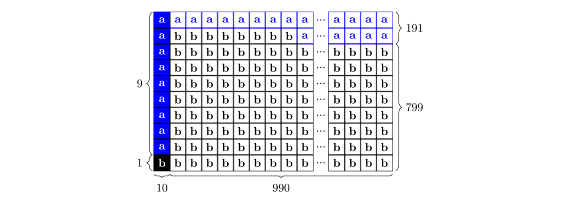
Figure 5 - Schematic representation of the example population of 1000 assets
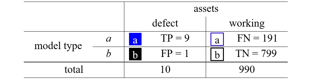
Table 1 - Confusion matrix of the example asset population
The a priori probability of a failure for one of the assets is known with p(H)=1 %. The proportion of defective assets of model type a to all defective assets describes (cf. (22)), while
is the proportion of working assets of model type a to all working assets (cf. (23)).
(22)
(23)
Then Bayes' theorem updates the a priori probability, which leads to a failure probability of of an asset after seeing the evidence that the asset is of model type a.
(24)
Equally, the calculation is possible using odds.
(25)
(26)
The model provides versatility, which is necessary for the utilities to meet the needs of their different demands and available data through the possibility of using various kinds of information as evidence and combining the evidence.
4. Exemplary application on a circuit breaker
In the following, the procedure is exemplified on a circuit breaker, whereby the versatility and the development of the basic structures for risk-based maintenance are demonstrated. A circuit breaker allows retrieving similar or analogous procedures for other high-voltage assets because measurements are performed regularly (although the intervals are often quite large with a few years), failures occur, and comprehensive and comparable literature is available, especially reliability surveys and FMEA. The circuit breaker is a live tank filled with SF6-gas, self-compression type, spring-load actuator, 420 kV rated voltage, and built 15 years ago by manufacturer Z. The example starts with a low-level risk assessment and increases in complexity while orienting on the maintenance strategies CM, TBM, and CBM. The probability and the consequences are assessed, but the focus lies on probability and the update with Bayes' theorem. For simplification, it is assumed that the risk calculation in the following is based on only one failure event.
4.1. Corrective Maintenance
A risk assessment based on a CM strategy for the circuit breaker is a low-level approach. The probability can be obtained through the annual failure rate. For live tanks rated 300 kV ≤ U ≤ 500 kV, while considering only major failures (MaF), the failure rate is λ =1.13 % (cf. Table 2.21 in [43]). Together with the replacement costs, which are about crep=200 000 € [44], the risk rCM is calculated (27).
(27)
This risk value has a limited informative value. Maintenance measures will still be triggered by a failure, but the value can be used to plan annual maintenance costs. Further, prioritisation can be made to locate spares when more circuit breakers are assessed. Evolving the risk value by considering more consequences or aggregating the risk to a higher (e.g. substation) level will make the prioritisation even more useful.
The advantage of the procedure arises when new information is available and implemented. Comparing the manufacturers internally within TenneT’s circuit breakers population shows that the failure rate of manufacturer Z is about 40 % higher. Manufacturer Z shares 8 % of the circuit breaker population. Considering a total population of 2800 live tanks (rated 420 kV), failures are expected. The failure rates of the other 21 manufacturers are nearly equally distributed. Therefore, 1.41 failures are expected for each manufacturer, respectively 1.98 for manufacturer Z. An update of the probability can be made analogously to section 3.3.
(28)
(29)
(30)
The new probability after seeing the evidence is λE=5.3 %, which results in the risk . In this way, the risk can be used as a trigger for maintenance measures. It is worth noting that with the update of the probability through Bayes' theorem, there is a shift from a general perspective of the whole population to an individual point of view.
4.2. Time-based Maintenance
For RBM based on TBM, the failure probability needs to vary over time. In absence of a failure probability function over time for the circuit breaker and inspired by [45], the probability function λ1 in (31) is assumed, with a=40 years as the expected lifetime of the circuit breaker and λ 0=1.13 % as the basic probability obtained above. Parameters may be changed or added to adjust the curve in real applications. The function has the advantage that it first exponentially grows but then approaches asymptotically the value 1, like the physical behaviour of a failure, which increases in probability as the condition worsens but will not exceed the probability 1 (cf. Figure 5).
(31)
Therefore, for the t=15 years old circuit breaker the failure probability would be and thus the risk with regard to the replacement costs is
.
Also, the time-dependent probability can be updated when new information is available, as the following fictional scenario shows: A investigation possibly finds that a seal, when older than 12 years, is responsible for 70 % of the failures, while in 5 % of the cases, it was not. Then Bayes' theorem can be used to update the failure probability of the t=15 years old circuit breaker.
(32)
But also, the complete failure rate function can be updated as in (33) so that
(33)
The probability for the 15 years old circuit breaker is also Both ways lead to the new risk quantified as
.
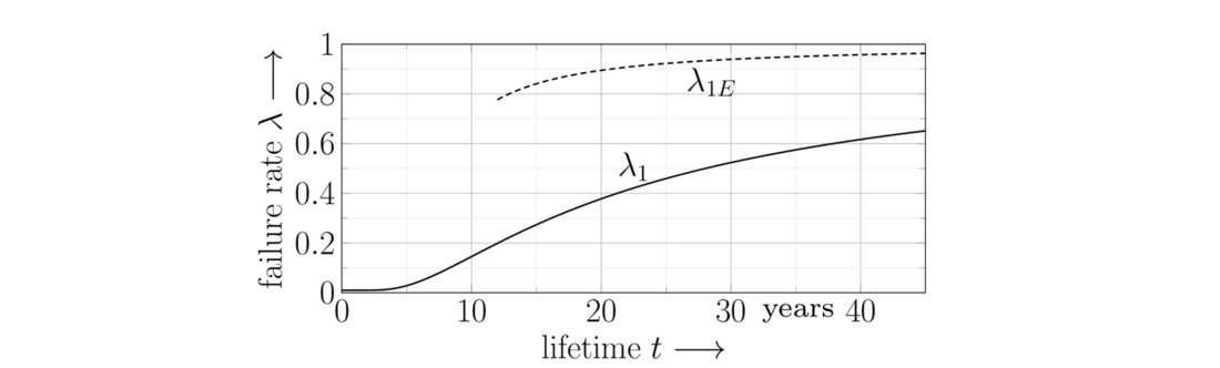
Figure 6 - Possible failure rate of a circuit breaker before λ1 and after seeing evidence λ1E plotted over lifetime t
4.3. Condition-based Maintenance
The CBM strategy triggers and prioritises maintenance measures depending on the condition of an asset. The condition is all information necessary to describe the current properties of a system. In the context of electric power supply, the condition can describe simplified functional capability since reliability is the superior objective. Therefore, a risk-based approach needs to assess the probability of a system to fulfil its function. The IEEE Standard Association provides in Std. C37.10.1 a general FMEA for circuit breakers [46], and WG A3.06 has surveyed in TB 510 the reliability of circuit breakers [43].
In the following, a scenario consisting in installing a monitoring system is presented. The monitoring system M measures gas pressure and density permanently. Then the effects on MaF and MiF are assessed. Since no statistic to M is available, it is assumed that M can identify 99 % of failure connected to a reduced gas pressure and density before they occur. M has a rate of 3 % for a false negative indication of a failure.
4.3.1. Minor Failure
For circuit breakers rated 300 kV ≤ U ≤ 500 kV the probability of a MiF is 9.3 % [43]. Further, a small SF6 leakage causes 35.6 % of the minor failures [43]. Therefore, the a priori probability of a MiF detectable by M is 3.26 %. Then Bayes' theorem allows calculating the failure probability when the information or evidence of the monitoring system is used.
(34)
So, an installed monitoring system M, which indicates a failure, leads to a failure probability of 52.7 %. Therefore, M adds 49.4 % certainty that a failure is present. Integrated into RBM, the failure probability is changed through an installation by, here reduced and thus -49.4 % (cf. (35)).
(35)
As a consequence of a minor failure, it is hypothesized that a technician has to travel to the substation and initiate a maintenance measure, for which costs of 5 000 € are assumed. The installation of M changes the risk with regard to MiF by -2 470 € (36).
(36)
4.3.2. Major Failure
For circuit breakers rated 300 kV ≤ U ≤ 500 kV the probability of a MaF is 1.13 % [43]. A rough calculation is used to estimate the a priori probability of a MaF detectable by the monitoring system: Monitoring the gas pressure and density enables the detection of 9 out of 90 failure causes stated in IEEE Std. C37.10.1 [46]. The failure modes in C37.10 and TB 510 are not identical. Nevertheless, the failure modes F1 "Does not close on command" and F2 "Does not open on command" are comparable. For a spring-type operating mechanism, these two failure modes share 76.4 % of all failure modes. Since F1 and F2 are not directly linked to the gas pressure or density, the monitoring system is not able to detect them. So vice versa, it is simplified assumed 23.6 % of the failure modes can be detected by M. The a priori probability of a MaF detectable by M thus is 0.27 %. Bayes' theorem leads to a posteriori probability for a MaF of 8.1 % (cf. (37)).
(37)
Analogue to (35), the change of M on the major failure probability is calculated in (38).
(38)
Estimating the risk in the simplest case that a major failure only leads to a replacement of a circuit breaker means a risk reduction by 15 684 €.
(39)
In total, the monitoring system M changes the risk by (cf. (40)), where
is the risk caused by the monitoring system, e.g. installation and operation costs. As long as
is negative, the risk is reduced, and the monitoring system is beneficial. In this case,
has to be smaller than 18 154 €.
(40)
The example shows that although the monitoring system is able to prevent 99 % of the failures, the usage strongly depends on either a high a priori failure rate or severe consequences, which is logical, but the presented approach enables to quantify usage as soon as the true positive and false positive rates are known. Analysing failure modes and accessing their probability allows a detailed condition assessment, but the effort of such an analysis is not neglectable.
The example illustrates that the risk has to vary to be used as a trigger. Further, prioritisation can be made when more than one risk is assessed. The decision-making becomes more objective, especially when different risk mitigation options are compared. The presented approach makes it possible to consider various kinds of information and implement this information as new evidence. In this way, the general perspective shifts to an individual view.
On the downside, it is not always easy to get the conditional probabilities required for an update using Bayes’ theorem. The versatility shown on equivalent CM, TBM, and CBM demonstrates the suitability for the individual needs of the different utilities.
5. Conclusion
A Bayesian risk-based maintenance approach is adopted on high-voltage assets. RBM is interpreted to include other maintenance strategies, thus having the advantage that utilities can retain pre-existing maintenance procedures. The basic model calculates a risk of an asset failure out of the failure rate and the consequences occurring from this failure. Then, the probability is updated when new information is available. For this, a failure hypothesis is made and the information declared as evidence updates the probability of the failure using Bayes' theorem. As a result, the probability, and therefore the risk, is better quantifiable, leading to more objective decision-making. In addition, a shift occurs from a population-based perspective of the probability to an individual one. This approach is advantageous because of versatility, which is reached by enabling the use of different kinds of available information and combining this information until sufficient certainty is reached. Thereby, the depth of the analysis can vary from simple to detailed. That way, the needs and the characteristics of different utilities and assets are respected. Further research is required in transferring knowledge into evidence usable for Bayes' theorem.
Acknowledgment
The authors would like to acknowledge the valuable contribution of Mr. Tobias Rodler from TenneT, who is a proven expert on circuit breakers.
References
- The German TSOs, „Grid Development Plan 2035 (2021),“ [Online].
- WG A3.30, “Substation equipment overstress management,” TB 816, CIGRE, Paris, 2020.
- S. Sahoo, P. Weitz, H. Schnittker, Y. Zhang, H. G. Bender, and C. Zeidler, "Improved health assessment of Substation using holistic condition monitoring," in ETG-FB. 163: ETG Kongress 2021, pp. 1-6, VDE, 2021.
- “Regulation (EU) 2019/941 of the European Parliament and of the Council of 5 June 2019 on risk-preparedness in the electricity sector and repealing Directive 2005/89/EC,” in Official Journal of the European Union, Vol. 62, 14. June 2019
- Übertragungsnetzbetreiber, Anhang zum Netzentwicklungsplan Strom 2035, Version 2021, zweiter Entwurf, [Online]
- M. J. Ashworth, “Ashworth, Michael J. "Preserving knowledge legacies: workforce aging, turnover and human resource issues in the US electric power industry,” in the International Journal of Human Resource Management, vol. 17, no. 9, pp. 1659-1688, 2006.
- “Asset management – Overview, principles and terminology,“ ISO 55000:2014.
- H. Schnittker, P. Werle, M. Rohleder, G. Bender, and M. Lottner, "Möglichkeiten des Einsatzes aktueller Monitoring-Systeme von Leistungstransformatoren zur Unterstützung des Asset Managements," in Proc. VDE High Voltage Technology, pp. 412-417, 2020.
- M. Schenk, “Instandhaltung technischer Systeme,“ Berlin, Springer-Verlag, 2010.
- R. D. Ross, “Reliability analysis for asset management of electric power grids,” Hoboken, Wiley/IEEE Press, 2018.
- J. Moubray, “Reliability-centered maintenance,” Industrial Press Inc., 2001.
- Analysis techniques for system reliability Procedure for failure mode and effects analysis (FMEA), IEC 60812, Beuth-Verlag, 2006.
- WG C1.16, “Transmission asset risk management,” TB 422, CIGRE, Paris, 2010.
- Risikobasierte Inspektion, DIN EN 16991, Beuth Verlag, 2018.
- H. Schnittker, P. Werle, L. Zha, M. Rohleder, and G. Bender, "Survey on asset management strategies of eletric grid operators," in Collection of ISH 2021 - 21th International Symposium on High Voltage Engineering, 2021.
- WG A2.49, “Condition assessment of power transformers,” TB 761, CIGRE, Paris, 2019.
- GB Distribution Network Operators, “DNO Common Network Asset Indices Methodology,” 2021, [Online]
- WG B3.48, “Asset health indices for equipment in existing substations,” TB 858, CIGRE, Paris, 2021.
- A. Azmi, J. Jasni, N. Azis, and MZA Ab. Kadir, "Evolution of transformer health index in the form of mathematical equation," in Renewable and Sustainable Energy Reviews, vol. 76, pp. 687-700, 2017.
- L. Wang, M. An, Y. Qin, and L. Jia, "A Risk-Based Maintenance Decision-Making Approach for Railway Asset Management," in International Journal of Software Engineering and Knowledge Engineering, vol. 28, pp. 453-483, 2018.
- N. Arunraj, J. Maiti, “Risk-based maintenance—Techniques and applications,” in Journal of Hazardous Materials, vol. 142, pp. 653–661, 2007.
- “Risk management – Risk assessment techniques,” ISO 31010:2019
- W. Tschirk, “Statistik: Klassisch oder Bayes. Zwei Wege im Vergleich,“ Springer, Heidelberg, 2014.
- A. Kolmogorov, “Sulla determinazione empirica di una lgge di distribuzione,“ in Giornale dell’Istituto Italiano degli Attuari, vol. 4, pp. 83-91, 1933.
- C. M. Bishop, “Pattern recognition and machine learning,” New York, Springer, 2009.
- P. Weber, G. Medina-Oliva, C. Simon, and B. Iung, "Overview on Bayesian networks applications for dependability, risk analysis and maintenance areas," in Engineering Applications of Artificial Intelligence, vol. 25, pp. 671-682, 2012.
- L. Leoni, A. Bahoo Toroody, M. M. Abaei, F. De Carlo, N. Paltrinieri, and F. Sgarbossa, "On hierarchical bayesian based predictive maintenance of autonomous natural gas regulating operations," in Process Safety and Environmental Protection}, vol. 147, pp. 115-124, 2021.
- E. Arzaghi, M. Abaei, R Abbassi, V Garaniya, C. Chin, and F. Khan, “Risk-based maintenance planning of subsea pipelines through fatigue crack growth monitoring,” in Engineering Failure Analysis, vol. 79, pp. 928-939, 2017.
- A. Eleye-Datubo, A. Wall, A. Saajedi, and J. Wang, “Enabling a Powerful Marine and Offshore Decision-Support Solution Through Bayesian Network Technique,” in Risk Analysis, vol. 26, no. 3, 2006.
- R. Abbassi, J. Bhandari, F. Khana, V. Garaniya, S. Chai, ”Developing a Quantitative Risk-based Methodology for Maintenance Scheduling Using Bayesian Network,” in Chemical Engineering Transactions vol. 48, pp. 235-240, 2016.
- G. Wang, T. Xu, T. Tang, T. Yuan, and H. Wang, “A Bayesian network model for prediction of weather-related failures in railway turnout systems,” in Expert systems with applications, vol. 69, pp. 247-256, 2017.
- D. Straub, "Stochastic modeling of deterioration processes through dynamic Bayesian networks," in Journal of Engineering Mechanics, vol. 135, pp. 1089-1099, 2009.
- S. Apeland, and T. Aven, “Risk based maintenance optimization: foundational issues,” in Reliability engineering & system safety, vol. 67, no. 3 pp. 285-292, 2006.
- F. Khan, M. Haddara, and S. Bhattacharya, “Risk‐based integrity and inspection modeling (RBIIM) of process components/system,” in Risk Analysis: An International Journal, vol. 26, no. 1, pp. 203-221, 2006.
- M. Muratović, K.Sokolija, and M. Kapetanović, “Modelling of high voltage SF6 circuit breaker reliability based on Bayesian statistics,” in Proc. 7th IEEE Conference and Exhibition (GCC), pp. 303-308, 2013.
- J. Sørensen, “Framework for Risk-based Planning of Operation and Maintenance for Offshore Wind Turbines,” in Wind Energy, vol. 12, pp. 493-506, 2009.
- M. Dirbaz, M. Modares and J.Mohammadi, “A Bayesian updating approach for bridge condition assessment using visual inspection data,” in International Journal of Structural Engineering, vol. 7, p. 127, 2016.
- T. Shindo, T. Takahashi, T. Okamoto, and T. Kuraishi, “Evaluation of Diagnostic Results by Bayes’ Theorem,” in IEEJ Transactions on Electrical and Electronic Engineering, vol. 7, pp. 450-453, 2012.
- M. Kallen, and J. van Noortwijk, “Optimal maintenance decisions under imperfect inspection,” in Reliability Engineering and System Safety, vol. 90, pp. 177-185, 2005.
- A. Tversky and D. Kahneman, "Judgment under Uncertainty: Heuristics and Biases," in Science, vol. 185, no. 4157, pp. 1124-1131, 1974.
- G. Sanderson, Bayes' theorem, 2019, [Online].
- S. Raschka and V. Mirjalili, “Machine Learning mit Python und Scikit-Learn und TensorFlow: Das umfassende Praxis-Handbuch für Data Science, Predictive Analytics und Deep Learning,” MITP-Verlags GmbH & Co. KG., 2017.
- WG A3.06, “Final Report of the 2004-2007 International Enquiry on Reliability of High Voltage Equipment,” TB 510, CIGRE, Paris, 2012.
- G. Balzer, K. Elves, H. Haubrich, C. Neumann, and C. Schorn, “Selection of an optimal maintenance and replacement strategy of HV equipment by a risk assessment process,” CIGRE Session, vol. 41, REF B3-103_2006, 2006.
- WG C1.1, “Asset Management of Transmission Systems and Associated CIGRE Activities,” TB 309, CIGRE, Paris, 2006
- IEEE Guide for the Selection of Monitoring for Circuit Breakers, IEEE Std. C37.10,1, 2018.