Method for the site-specific conversion of weather parameters for probabilistic calculations of OHLs
Authors
S. STEEVENS, E. ULLOA JIMENEZ, C. ENGELKE - Amprion, Germany

Summary
The determination of the weather parameters are essential for a site-related probablistic calculation of an overhead line pylon and for the calculation of the current carrying capacity. As a rule, these parameters are not measured directly at each pylon location, consequently extrapolation or conversion methods must be used.
In Germany, the weather parameters are recorded in a narrow geographical grid by the German Weather Service (DWD) and made available via a homepage. The data are usually available as hourly values with a sufficient observation length. With the help of that data, an optimised determination of the steps for the static calculation on each pylon can be achieved. For the weather parameters air temperature, global radiation, relative humidity, air pressure, precipitation and dew point temperature the ordinary kriging method is used, whereby in the case of air temperature and dew point temperature a further extrapolation must take place on the basis of the height difference.
To extrapolate the wind data, a sector-dependent macro wind climate is created for the route of the OHLby adjusting or homogenising the wind measurement data (mean wind speed) using the topography and ground roughness at the measurement location (weather station). Subsequently, the wind gust speeds required for dimensioning can be determined at the pylon location by taking the topography and ground roughness into account in the same way as for the weather station. The now pylon-specific extrapolated weather data can be used, for example, to determine sector-dependent ice and wind loads.
To validate the method, this paper compares the extrapolated values of the respective weather parameters with the actual measured values. The extrapolated values are based on data retrieved from the German weather service. The values used as reference were recorded on sensors, which were either mounted on an overhead line pylon or in a substation of Amprion GmbH. In this way, it was not only possible to validate the procedure, but also to differentiate the influence of individual boundary conditions, such as topography and ground roughness. In summary, it can be said that, provided that sufficient input data from weather measuring stations are available, the models presented allow very good data extrapolations, consequently the data obtained can be further processed for further probabilistic verifications. These approaches serve for the site-specific conversion and determination of distribution functions, which can then be used for probabilistic verifications
Keywords
ordinary Kriging - Extrapolation of weather parameters - sector-dependent annual extreme value of wind speed, ambient temperature - dew point temperature - global radiation - relative humidity - precipitation1. Introduction and goal
For the static calculation of overhead line pylons and the electrotechnical design, weather parameters play an important role in high and extra high voltage overhead lines. With precise site-related knowledge, more exact external loads can be calculated, which leads to a load factor that is appropriate to the site. In particular, by applying the probabilistic method for pylons calculations (see [1]), more exact utilisation can be determined for pylons due to the presence of the site-specific loads. This makes optimal use of existing reserves and guarantees a sufficient level of safety. With the focus on electrical loads, site-specific weather data can also identify existing reserves and possibly even lead to an increase in the maximum transmission capacity, as is already made possible by weather-dependent grid operation.
In the following, the site-specific conversion methods of the relevant weather parameters required for this are explained and described. The weather parameters air temperature, global radiation, precipitation, relative humidity and humidity temperature can be converted according to the Ordinary Kriging method. The conversion of the wind speed is essentially carried out according to the wind standard [2] and [3].
It was shown in [4] that the wind speed strongly depends on the location. Therefore, a conversion from the measurement location to the relevant location of the overhead line is mandatory. Local conditions must be taken into account for the conversion. Important local conditions in this context are the roughness and topography resulting from the terrain geometry. Furthermore, the different altitude above sea level were taken into account. In general, a terrains use is divided into roughness classes, consequently a height profile of the wind speed can be characterised via a roughness length assigned to the classes. This approach is used, for example, in the utilisation of wind energy. Furthermore, it can be transferred to the utilisation of an overhead line, as similar heights close to the ground surface can be assumed in this context.
2. Theory for the site-specific conversion of weather parameters
2.1. Ordinary Kriging Method
The Ordinary Kriging method can be interpreted as a geostatic method for interpolating spatial data. Basically, this method is based on the idea that two spatially close points have similar values. A spatial correlation is thus assumed, with which variations on the surface can be taken into account. As an alternative method, the inverse distance weighting method exists, which, however, does not take the spatial variance into account. The spatial variance is taken into account by the so-called semivariograms, consequently not only an optimal prediction of the values at the locations to be considered can be made, but additionally a confidence measure for the predicted values is provided.
2.1.1. Structural analysis
The Ordinary Kriging procedure thus not only provides an optimal prediction, but also provides a confidence measure for how likely this prediction will be true. In the first step of the Kriging method, the structural analysis for spatial modelling must first be carried out. For this, the semivariance is determined. Mathematically, the semivariance is defined as:
(1)
With
: Semivariance
di : distance
z(i) : Value of the variable at location i
z(x) : Value of another variable with distance
i : Index to a place
n : Number of values for a location with the distance
The semivariogram (see Figure 1) can be plotted from the values of the semivariance (di ). This shows half the average squared difference between two units. If pairs of points have the same distance, they can first be grouped into so-called distance classes and then be displayed.
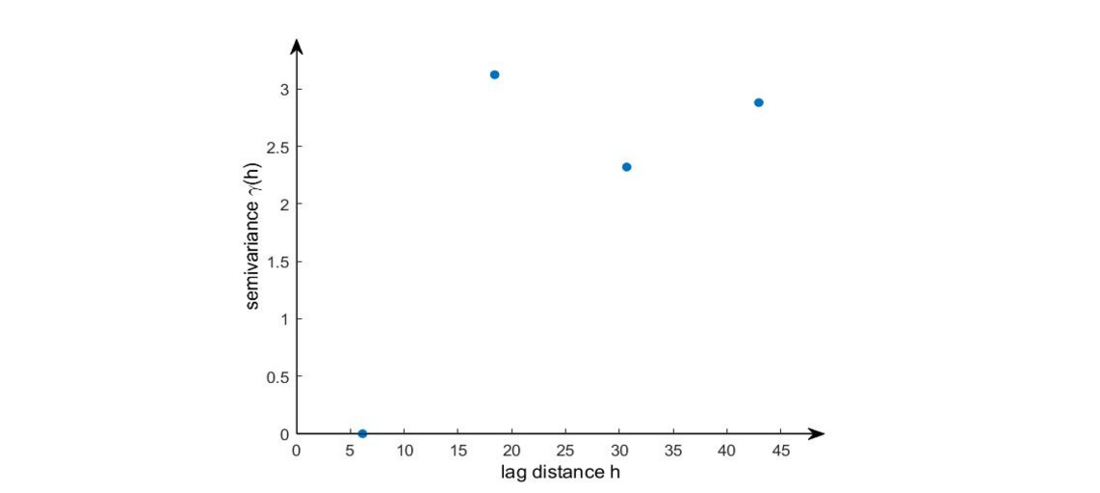
Figure 1 - Example semivariogram
In principle, it is to be expected that in a spatial correlation, points that are closer together have similar values than those that are further apart. For a semivariogram this means that in principle with larger x-values the squared differences become larger and thus more dissimilar.
2.1.2. Model fitting
With the help of this empirical semivariogram, the next step is to adjust the model, consequently a spatial description and spatial prediction is possible. In doing so, the empirical semivariogram can be used to identify information on the spatial correlations. For this purpose, the three characteristic features of a theoretical semivariogram are determined. These are shown in the following figure:
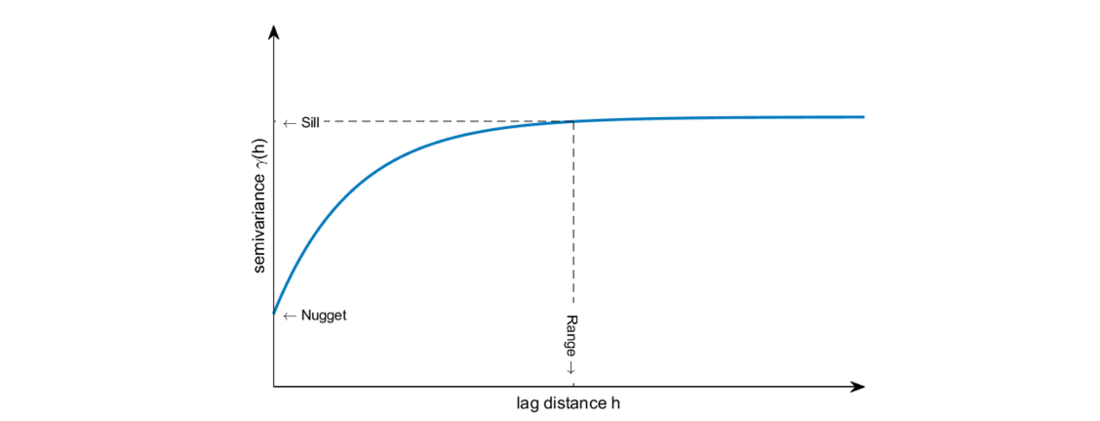
Figure 2 - theoretical semivariogram
In this, the so-called "nugget" indicates a measure for the scattering of the signal in the near range (measurement error). The "range" describes the spatial area in which the points correlate to each other (range of information). In this range, an interpolation makes sense and thus leads to good results. The threshold value "Sill" describes the maximum of the semivariogram.
Then a substitute function must be chosen that approximates the calculated values of the semivariance (di ) as closely as possible. In principle, circular, spherical, exponential, Gaussian and linear substitute functions are available as shown in the following figure:

Figure 3 - possible theoretical substitute functions for the semivariogram
- Spherical model: The spherical model is the most frequently used model. It increases linearly at the origin and reaches sill C at distance a.
- Exponential model: The exponential model follows an exponential function. The range a is reached very slowly. - typical for soil humidity values.
- Gaussian model: rises very flat, favourable for very continuous variables with relatively small nugget effect.
The fixed model approach influences the prediction of the values to be determined in such a way that the function values of the substitute function in the vicinity of the coordinate origin should meet the values of the empirical semivariogram as close as possible, otherwise the values will differ greatly.
2.1.3. Determination of the prediction
After the model fitting step, a prediction will be made. For this, as with other methods, a weighting must be determined, consequently neighbouring measured values can be transferred or predicted to a non-measured position. For this purpose, the estimation variance is first established according to [5]:
(2)
To determine the weighting , three constraints must first be established:
- Estimation error is zero on average:
(3)
- Variance E of the estimation error is minimal:
(4)
- Sum of the weights
is 1:
(5)
With these constraints on the estimation variance, the so-called Ordinary Kriging Matrix can be set up:
(6)
With
 : Weighting to the data values
 : Lagrange parameter
In general terms, this can be formulated as:
(7)
The values for the matrix [A] and the vector [B] can be taken directly from the semivariogram. Then, with the help of this Lagrange equation system, the parameters for the weighting can be determined. Subsequently, the values sought can be calculated on the basis of these weightings and the associated estimation variance can be determined. It can be stated that the lower the estimation variance, the better the estimation.
2.2. Method for converting wind speeds
The following procedure is used to create a direction-dependent stochastic model to determine the probabilistic wind effect for the calculations of the pylons. For this purpose, the annual extreme values of the mean wind speeds measured at nearby weather stations are first converted to standard reference conditions. Based on the adjusted data, suitable probability distributions are created that describe the regional climate (macroclimate). Subsequently, a profile of wind gust speeds can be created for the probabilistic wind load approach, taking into account the terrain properties (ground roughness and topography). Furthermore, this approach can be transferred to the hourly average values so that these converted values can be used as a further input variable (e.g. for the current carrying capacity).
2.2.1. Extreme value distribution
For the probabilistic verification of pylons in existing structures, the parameters of a probability distribution of wind gust speeds are subdivided into 15° sectors (24 circular sectors) for each pylon and the respective wind frequency at the site is to be calculated. The distribution is generated from the wind speeds and wind directions measured at neighbouring weather stations of the German Weather Service (DWD). An extreme value analysis lists the annual maximum values of the mean wind speed for each sector the stochastic representation of which can be produced by an extreme value distribution (Gumbel type III).
The Gumbel distribution type III differs from the standard Gumbel distribution (type I) by an upper limit of the recorded data, which has a probability of undercutting of 1. This is evident for wind data, as wind speeds cannot physically be infinitely large. The determination of an upper limit gives the distribution a further parameter in addition to the expected value and the standard deviation with the curvature .
The distribution sum function is defined as follows:
(8)
With:
: Expected value
: Standard deviation
: Curvature parameter
(9)
(10)
Gamma function:
(11)
The Moment Method is suitable for parameter estimation due to the large amount of data usually available. The method estimates the moments ms and from the sample x1 to xn with sample size n, which are approximately equal to the distribution parameters.
- Expected value
(12)
- Standard deviation
(13)
The third parameter can be determined by estimating the parameter
. Another approach is to estimate the curvature by its relationship with the distribution upper limit Xmax. To determine an upper limit of the mean wind speed in Germany, the wind measurement data of the weather stations of the German Weather Service were used as a basis. The weather stations are available in sufficient density that their data evaluation can be considered representative for all wind zones in [3].
(14)
| Wind zone | 1 | 2 | 3 | 4 |
|---|---|---|---|---|
Xmax [m/s] | 50.988 | 56.654 | 62.319 | 67.984 |
2.2.2. Data analysis and processing
For the statistical evaluation of the wind conditions in the region under consideration (macroclimate), the wind measurement data at the weather stations are available as 1h mean values with the respective wind direction. The annual maximum values are determined from the measured data and divided into 30° sectors (Figure 4) with the help of the indicated direction.
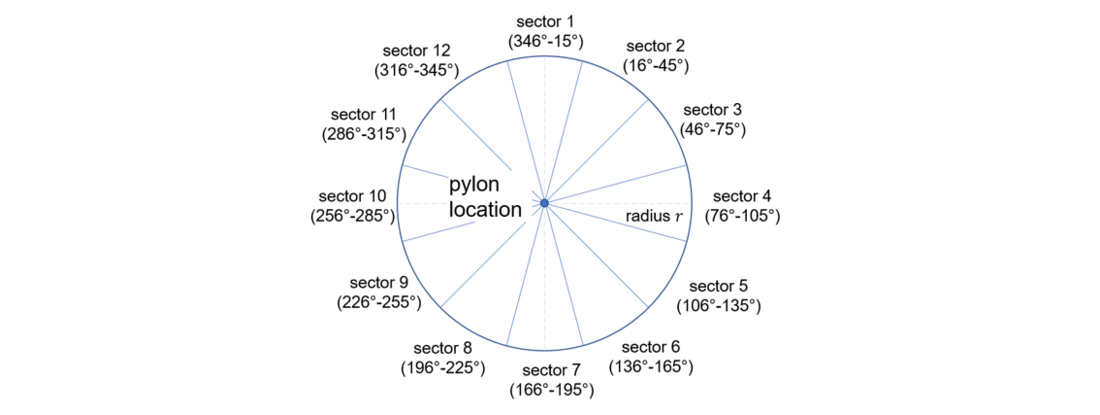
Figure 4 - Sector split
Since the 10-minute wind speeds are required to determine the acting wind loads, the 1h mean values must be converted by a factor of 1.04 to 1.08 (see [4] and [6] ()). In addition to the annual extreme values of the mean wind speed, the frequency distribution of the wind speed and wind direction is calculated in 30° sectors. For this purpose, the wind speeds are recorded in steps of 1 m/s.
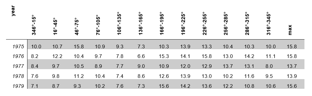
Table 2 - Example of annual extreme values of the 10 minutes mean wind speeds in m/s for a 30° sector split (5-year section)
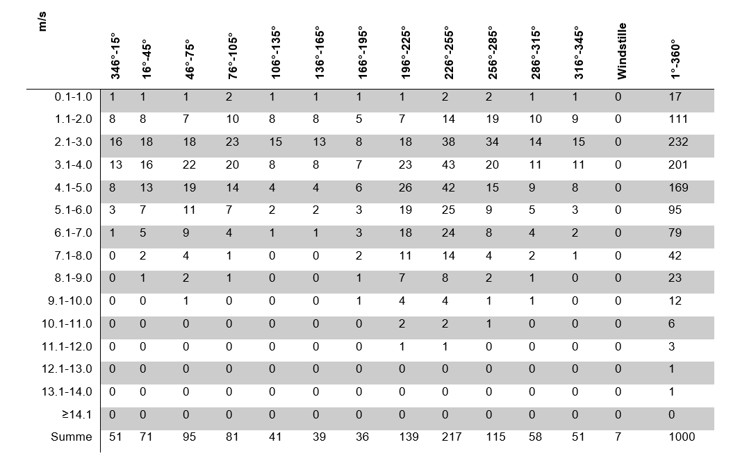
Table 3 - Example frequency distribution of wind speed and direction in ‰ for a 30° sector
2.2.3. Data homogenisation
The basic value of the base wind speed is the direction-independent characteristic value of the mean 10-minute wind speed. Its exceedance probability is 0.02 and thus a statistical return period of 50 years (1/0.02). This refers to 10 m height above ground on level, open terrain with low vegetation (roughness length z0 = 0.05 m). This corresponds to terrain category II according to DIN EN 1991-1-4/NA (standard reference condition). The basic value of the base wind speed is determined in Germany by the four wind zones according to [3]. Using the method presented here, significantly smaller values than in the standard can be achieved. The basic wind speed
captures the relationship between wind strength and wind direction
and is dependent on the basic value of the basic wind speed
.
(15)
A value of 1.0 is recommended for both the directional factor cdir and the seasonal coefficient cseason, consequently the wind load is determined based on the basic value of the base wind speed.
For all weather stations used to determine the wind load impact, the base wind speed in the 30° sectors is determined as the 0.98 quantile value of the annual extreme values.
The 10-minute values obtained by the conversion in chapter 2.2 must consequently be converted to the standard reference conditions
 . This is done with the help of the profile of the mean wind speed per sector:
(16)
(17)
With:
: Topography coefficient for the mean wind
: Terrain factor (interpolated to Z0)
: Profile exponent (interpolated to Z0
 )
)
z : Altitude above ground
DIN EN 1991-1-4/NA defines four terrain categories that based on the roughness length Z0. The terrain factor and the profile exponent are assigned to the respective terrain categories (see Table 4), consequently the values matching any roughness length Z0 can be determined by interpolation. The exact calculation of the roughness length present in each sector is presented in chapter 2.2.6. The topography coefficient present in each sector is determined according to [2] A.3 (see chapter 2.2.7).
By transferring to the standard reference conditions, a stochastic model for the supraregional description of the wind climate (macro wind climate) can thus be created. The data are recorded sector by sector by the extreme value distribution Gumbel type III, whose parameters are determined by the moment method. For a realistic stochastic wind model, the influence of thunderstorms, which are not represented by the data measured at the weather stations, must also be taken into account (see chapter 2.2.4).
To illustrate the procedure, the theoretical and empirical distribution for a fictitious sector is presented below. A total of 40 annual extreme values are available for the random variable wind speed. Based on the moment method for parameter estimation and after data homogenisation for the macroclimatic representation of the wind conditions, the Gumbel distribution type III can be created.
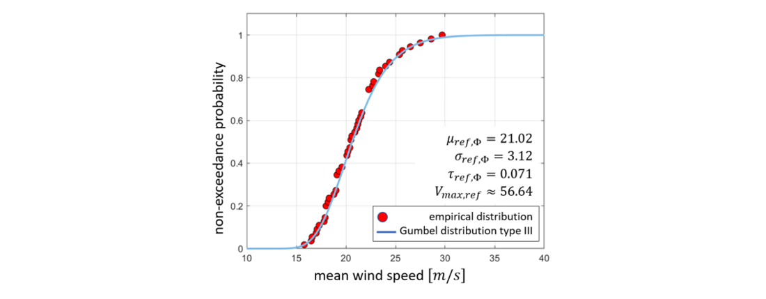
Figure 5 - Empirical distribution and Gumbel distribution type III for an example sector
The 98 % quantile value of the distribution after data homogenisation corresponds to the base wind speed . The parameters of this distribution are marked with the index „ref“ and are used in the following steps to determine the wind gust speed at the pylon site.
To validate the procedure of data homogenisation or extrapolation of the measured data on the macroclimate in the line environment, the extrapolated data are compared with the wind speeds actually measured at the pylon or at a site in chapter 3.
2.2.4. Consideration of thunderstorm events
Thunderstorms are caused by extremely large differences in temperature and humidity over height. They produce extreme wind gust speeds at comparatively low mean wind speeds. Therefore, the effects of thunderstorms are not present in the annual maximum values of mean wind speeds. To capture these effects, a thunderstorm-specific extreme value distribution is developed to provide a lower bound for each sector. The 0.98 quantile value of the thunderstorm distribution is calculated as 70 % of the 0.98 quantile value (50-year value) of the direction-independent distribution of mean wind speeds.
2.2.5. Conversion of the 30° sectors to 15° sectors
With regard to the probabilistic calculation of the overhead line towers, the determined 30° sector distributions are transferred to 15° sectors by interpolation between the neighbouring sectors. This is done for the wind speeds as well as for the wind frequencies.

Figure 6 - Example of interpolation in sector 4 from 30° sectors to 15° sectors (0.98 quantile value)
2.2.6. Calculation of the roughness length
The ground roughness is required both at the weather station site for data homogenisation of the measured wind data and at the pylon sites for correction of the wind gust speeds. In [3], a distinction is made between 4 terrain categories for which the roughness length has already been determined. In addition, the terrain factor fg and the profile exponent are given for each category.

Table 4 - Terrain categories according to [3]
To determine the roughness length z0 at the site under consideration, the land use in the vicinity of the site is examined. A seamless land use map is provided by the European CORINE Land Cover [7], which covers the main forms of land use in Europe. The land use map is summarised into 9 categories with associated roughness lengths. The listed roughness parameters were assigned following the normalised and existing terrain categories.
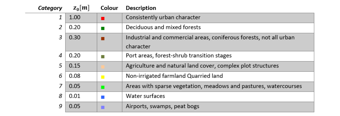
Table 5 - Roughness classes and associated roughness lengths
If individual pylon or line coordinates are available, the roughness lengths can be determined by analysing the individual pixels around the location. A circle divided into 12 sectors with the empirically determined radius is to be selected around the location under consideration. In each sector, a roughness length averaged over all 9 categories is then determined. By calculating the roughness lengths weighted by the number of category-related colour pixels in relation to the total number of pixels in the sector.
(18)
Thus, the corresponding roughness lengths can be determined for each sector, as shown by way of example:

Figure 7 - Representation of the roughness length in each sector within a radius of 3 km
After this determination of the roughness length for each sector, the terrain factor on the one hand and the profile exponent on the other hand can be interpolated between the above-mentioned terrain categories for the mean wind speed, the turbulence intensity and the wind gust speed. The turbulence intensity shows the deviation from the mean value of the measured wind speeds (
) and is further required to determine the topography coefficient of the wind gust speed.
2.2.7. Calculation of the topography coefficient
Another relevant factor for the conversion of wind speeds is the topography coefficient. This coefficient is needed to adjust the wind speed due to the local height profile to the site under consideration. If the site under consideration is located on a windward slope or on the crest of a hill, this can lead to an increase in wind speed and a decrease in turbulence intensity . Data from the Shuttle Radar Topography Mission (SRTM data) [8] are used to analyse this situation. The corresponding height information is available with an accuracy of 30 m. The topography is examined both at the weather stations for data homogenisation on the one hand and in the line environment for correction of the wind gust speed on the other.

Figure 8 - Topography for a sample line / Figure 9 - 3D topography at pylon 4
The examination is carried out analogously to the roughness in 30° sectors by creating a section through each sector. Since the terrain on the rear side of the pylon is important for the topography coefficient, the cut is always made across two sectors. For example, by looking at sector 5, sector 11 is also represented. The determination of the topography coefficient for the mean wind speed is carried out in the standard case according to Appendix A.3 in [2], while the reduced turbulence intensity can be determined according to Appendix NA.B in [3].
(19)
(20)
With:
: Mean wind speed at height z above ground (on the mountain)
: Mean wind speed over flat terrain (at the foot of the mountain)
: Turbulence intensity at the foot of the hill or slope
The geometric possibilities to capture the terrain elevation are more limited and can only be applied by simplifying the actual topography. As a result, the cuts made through the sectors are geometrically simplified based on their main points(start and end points, lowest points and highest points on both sides, pylon point and crest). In addition, the slopes of the lines between these points are used to identify the appropriate case according to [2] A.3 distinction is made between three cases:
- The location is in the windward area
- The location is in the leeward area (slope < 0.05)
- The site is located in the leeward area (slope > 0.05).
In addition, slopes smaller than 5 % are not considered relevant, consequently the topography coefficient takes the value 1.
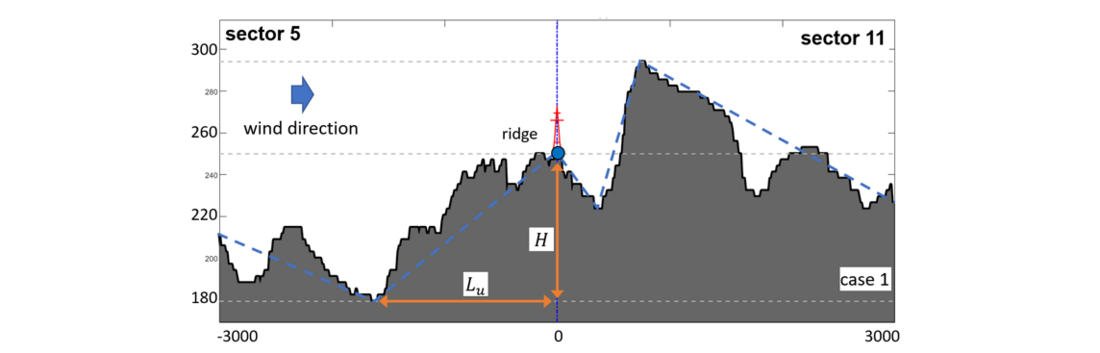
Figure 10 - Topography section for sector 5 and its simplification for the application of the calculation method according to [2] and [3]
The topography coefficient for the wind gust speed can be calculated according to the procedure of [2]. For this, the turbulence intensity at the foot of the hill or slope must be determined. This is done using equation (20) with known turbulence intensity
 , which can be calculated by interpolation depending on the location category.
(21)
The method according to [2] and [3] is best suited for isolated mountains, mountain ranges or slopes, consequently a critical consideration of the calculation results is necessary. For complex topographic profiles, a CFD simulation can be useful. An example for the validation of the method is calculated in chapter 3.
2.2.8. Gumbel distribution parameters for wind gust speed
After creating a macro-climatic model for wind speed and wind direction in the route of the OHL and by determining both the roughness coefficients and the topography coefficients to the wind gust speed, the distributions of the gust wind speed can be established.
(22)
With:
: Topography coefficient for wind gust speed
: Terrain factor (interpolated to z0)
: Profile exponent (interpolated according to z0)
z: Height above ground
After determining the reference distributions of the mean wind speed, the Gumbel III distribution parameters for the wind gust speed can be determined. The values for the frequency remain unchanged for the wind gust speeds:
(23)
(24)
(25)
(26)
With the calculated distribution parameters for all 24 sectors (15° sectors), the wind loads can now be recorded in the combinatorics for probabilistic calculation.

3. Case studies
In the following section, the theoretical procedures for the conversion of weather parameters explained above are presented using case studies. For this purpose, two parameters are compared in each case. On the one hand, a measured value at the location to be observed and, on the other hand, a corresponding converted value according to the above-mentioned procedures. The meteorological parameters are taken from weather measuring stations of the German Weather Service [9] as the data basis for the conversion. For comparison, measured values from pylons and substations of Amprion GmbH from the adaptive overhead line operation project are then used. Due to the availability of data from the Amprion sensors, the focus of these considerations should be on air temperature, global radiation, relative humidity, air pressure and wind speed.
3.1. Case study sensor A
In the first case study, the weather parameters air temperature, global radiation, relative humidity, air pressure and wind speed are converted to the site of sensor A and compared with real measured values at the site.
3.1.1. Calculation of the weather parameters air temperature, global radiation, relative humidity and air pressure
In the following, the results of the conversion of the weather parameters temperature, global radiation, relative humidity and air pressure according to the Ordinary Kriging methodology are presented. The starting point for this conversion is formed by the stations surrounding the location of sensor A (see Figure 11 on the left).
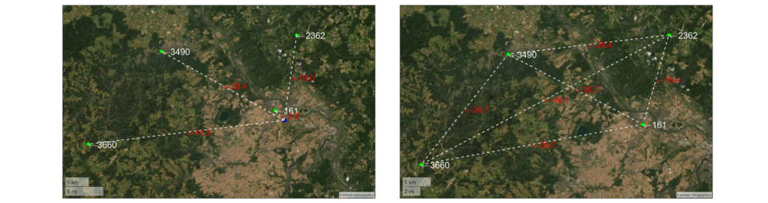
Figure 11 - Surroundings of the location of sensor A (blue dot) from Google Earth
Data for the conversion to the location under consideration can be used from the following stations (see Table 6):
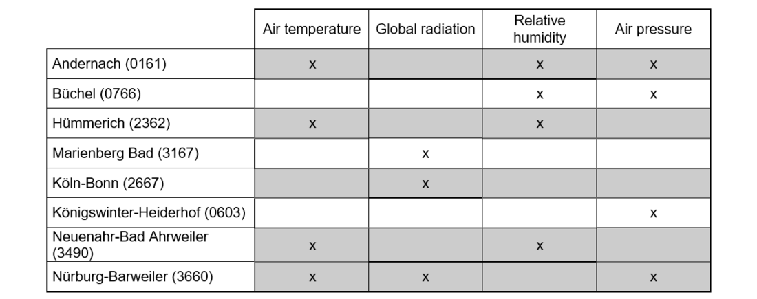
Table 6 - DWD stations for calculating the weather parameters at the location of sensor A
Based on these parameters, an exemplary conversion of the air temperature for the four stations Andernach, Hümmerich, Bad Ahrweiler and Nürburg Barweiler is carried out below, consequently the applicability of the methodology is made clear.
The distances between these locations and thus the basis for deriving the Ordinary Kriging Matrix are summarised in the following table:
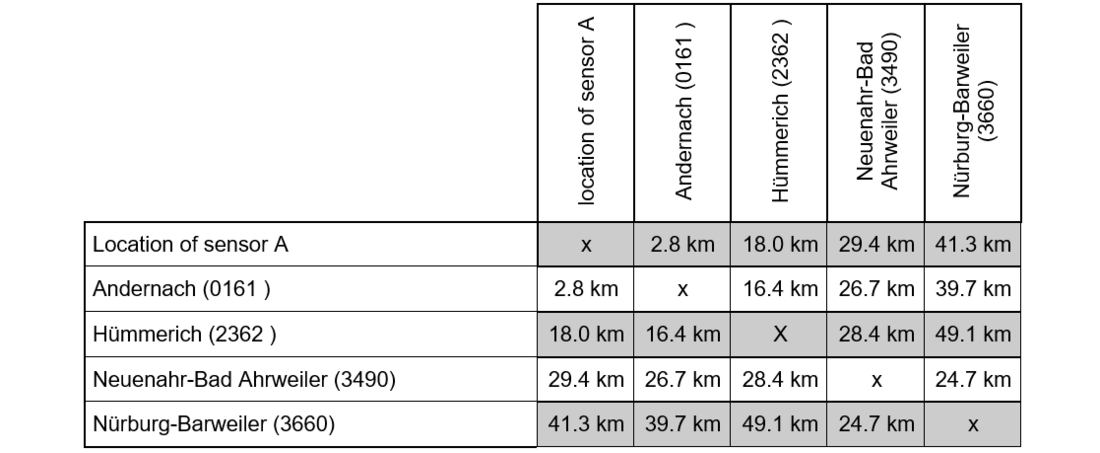
Table 7 - Distances of the sites for the calculation of the air temperature
With the help of the ordinary kriging method presented in chapter 2.1, the empirical semivariogram including the theoretical substitute function for a defined time (17 June 2021 01:00:00) can be determined for the location of sensor A:
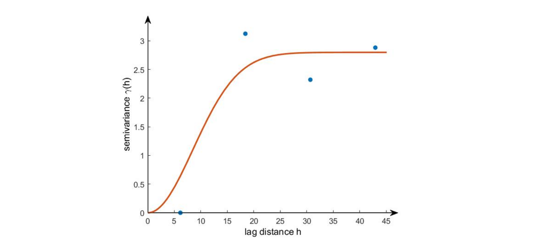
Figure 12 - Semivariogram including approximation function
Based on this semivariogram, the following substitute function can be determined:
(27)
With:
c0 = 0 , c = 2.7994 and a = 12.0238
Thus, the Ordinary Kriging Matrix can be set up as:
(28)
This results by inserting the corresponding distances:
(29)
This allows the weights to be determined:
(30)
Consequently, the expectation variance as a quality characteristic can be calculated to:
(31)
The conversion of the individual values to the relevant location can thus be carried out in each data point using the following equation:
(32)
Taking into account these determined weights, the temperature at the exemplary time of 17 June 2021 01:00:00 can thus be determined to:

Table 8 - Exemplary calculation of the air temperature
On the basis of this exemplary calculation of the air temperature with 13.613 °C and the comparison with the real measured temperature at the site of sensor A with 13.610 °C, it can be seen that the ordinary Kriging method provides acceptable values that can be used for further considerations.
With the help of the measured values of the sensor A in the period from May 2018 to February 2022, the synthetically generated values can be compared with the real measured values for a longer period and the deviations presented. These are compared in the following Figure 13:
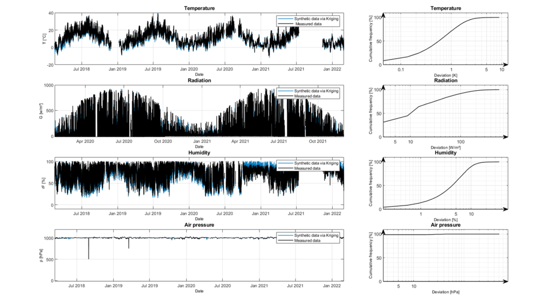
Figure 13 - Comparison of real measured values and synthetically generated ones at the location of sensor A
First of all, it must be mentioned that the data gaps in Figure 13 are due to missing measurements of sensor A. These were therefore not considered further for the comparison. Basically, four data series (air temperature, global radiation, relative humidity, air pressure) are shown with the respective deviations and their cumulative frequency distributions. It can be seen that the conversion of the air temperature to the location of sensor A with the help of the stations indicated in Figure 11 with approx. 70 % allows a deviation of less than 1 K. The global radiation values reach a deviation of less than 40 W/m2 to 80 % of all values. The relative humidity reaches an absolute deviation of less than 8 % at approx. 80 %. When converting the air pressure, it can be stated that the deviations are so marginal that it can be assumed that the air pressure is close to 100 %.
The stations used are located at different altitudes above sea level (sensor A: 120 m, 2362: 328 m, 3490: 111 m, 3660: 485 m), consequently a temperature adjustment is necessary due to the difference in altitude. This has been taken into account in Figure 13 with a value of 0.0065 K/m.
3.1.2. Calculation of the wind speed
In the following, the results of the conversion of the weather parameter wind are presented and a comparison is made between the sensor A and the DWD weather station. For this purpose, the average wind speeds of the sensor A and the DWD weather station in Andernach are evaluated and compared. The focus in this section is on the influence of roughness. The screenshot from Google Earth (Figure 11) shows an agricultural and partly urban character with relatively flat terrain.
Table 9 summarises the key data of both measuring stations. In the following comparison only sector 11 is explained, therefore the values for roughness and topography apply to this sector. The difference in roughness length z0 is clearly visible in this case. In Andernach this is 0.29 m and at the location of sensor A 0.08 m, consequently a difference of 0.21 m results. In contrast, the values for the topography coefficient co,vm for both measuring stations are 1.00. This means that the topography has no influence on the homogenisation of the values.
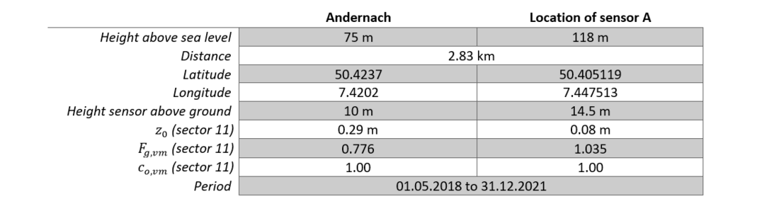
Table 9 - Data from the weather stations Andernach and the location of sensor A
Figure 14 shows sections of the land use map around the respective measurement sites. The weather station in Andernach (left) was considered with a radius of 600 m around the measurement site and the sensor A (right) with a radius of 870 m around the measurement site. The larger radius in the location of sensor A is justified by the connection between the height of the sensor at the measurement site and the choice of the radius to be considered.
The height of the sensor A, which deviates from the standard reference conditions, additionally influences the measured values, consequently the profile exponent m is used for data homogenisation.
Sector 11 is particularly suitable for comparison, since it is almost completely assigned to category 3 in Andernach and completely to category 6 in the location of sensor A (compare Table 5). When transferring to standard reference conditions, an adjustment of the values in the rougher sector 11 of the station in Andernach should therefore be observed, as expected.

Figure 14 - Representation of the roughness length in each sector (left: DWD weather station in Andernach, right: location of the sensor A)
Basically, it can be stated that the two data series for the annual extreme values in Figure 15 show similar or parallel courses over the entire period under consideration. As expected, the station in Andernach delivers the lower values due to the greater roughness of the terrain. In order to quantify the deviation of the two courses, the average of the monthly differences in wind speed is determined. The difference between the data are less than 1.9 m/s in 90 % of the values.
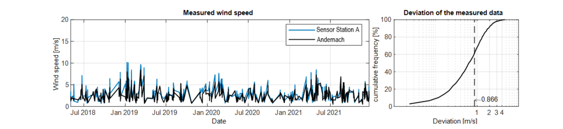
Figure 15 - Comparison of the measured annual extreme values of the 10 minutes mean wind speed for sector 11 (deviation: 90 % < 1.9 m/s)
Figure 16 shows the homogenised annual extreme values. When looking at the diagram, it is immediately apparent that, as expected, a convergence of the two curves has taken place. The difference between the data series is now 90 % of the values below 1.7 m/s. It is also worth mentioning that values from the sensor of station A have hardly changed, but only the values from Andernach have increased accordingly.

Figure 16 - Comparison of the homogenised annual extreme values of the 10 minutes mean wind speed for sector 11 (deviation: 90 % < 1.7 m/s)
3.2. Case study of sensor B on the pylon
In the second case study, the weather parameters air temperature, global radiation, relative humidity, air pressure and wind speed are converted to the location of a pylon (sensor B) and also compared with real measured values at the location. In contrast to the above comparison at the site ofsensor A, the sensor is located directly on the overhead line pylon. Furthermore, the distance between the measuring stations is significantly greater.
3.2.1. Calculation of the weather parameters air temperature, global radiation, relative humidity and air pressure
Figure 17 shows the stations used and the distances to the pylon site. Furthermore, the screenshot shows an agricultural and partly urban character with relatively flat terrain. However, the data history for this comparison only covers October 2021 to November 2021.

Figure 17 - Surroundings between Mönchengladbach-Hilderath and the location of the pylon (blue dot) from Google Earth
For this calculation of the weather parameters, data on the pylon under consideration can be used from the following stations:
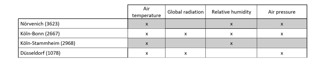
Table 10 - DWD stations for the calculation of weather parameters at location of sensor B
The calculation of the weather parameters air temperature, global radiation, relative humidity and air pressure show comparable percentage results despite the short data history. Figure 18 shows that the air temperature shows a deviation of less than 0.8 K in 80 % of cases. The global radiation values show only an absolute deviation of less than 20 W/m2 at a cumulative frequency of 80 %. The measurement of relative humidity shows a higher deviation than in the first case study with an absolute deviation of 10 % to 80 % of all values. The air pressure also achieves almost 100 % accuracy in the second example through the Ordinary Kriging methodology.
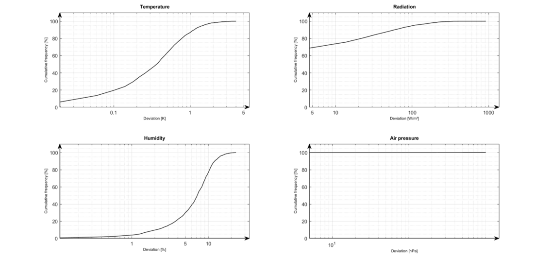
Figure 18 - Cumulated deviations of the real measured values and the synthetically generated values at the pylon location of sensor B
The stations used are located at different altitudes above sea level (sensor B: 58 m, 1078: 37 m, 2667: 92 m, 3968: 43 m, 3623: 100 m), consequently a temperature adjustment is necessary due to the difference in altitude. This has been taken into account in Figure 18 with a value of 0.0065 K/m.
3.2.2. Calculation of the weather parameter wind
In the following, a comparison is made between the wind speed of sensor B on a pylon and the weather measuring station Mönchengladbach-Hilderath of the DWD.
Table 11 summarises the essential boundary conditions. For sector 9 considered here, the roughness length around the pylon is twice as high as at the location of the DWD weather station. In the homogenisation of the values, the topography again plays no role, as the values in both cases are 1.00.
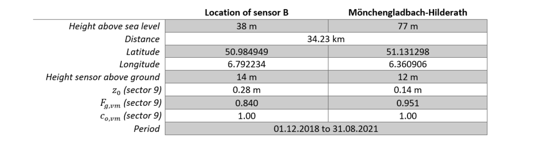
Table 11 - Data from sensor B on the pylon and the weather station of Mönchengladbach-Hilderath
The land use map in Figure 19 shows for sector 9 at the weather station in Mönchengladbach-Hilderath (left) a partial use of category 2 and partly as category 6. For sector 9 at the OHL pylon (right) a use of category 3 is shown almost continuously. When transferring to standard reference conditions, therefore, an adjustment of both data series must take place as expected, whereby the measured values from sensor B clearly approach the values of the DWD weather station.

Figure 19 - Representation of the roughness length in each sector (left: DWD weather station in Mönchengladbach-Hilderath, right: sensor B on the pylon)
In contrast to the measured annual extreme values from Figure 15, the values in Figure 20 show a similar level in the height of the measured wind speed, but a not so high parallelism of both courses. There is therefore a correlation between deviation and distance of the recording sites. The data series differ by less than 2.3 m/s in 90 % of cases.
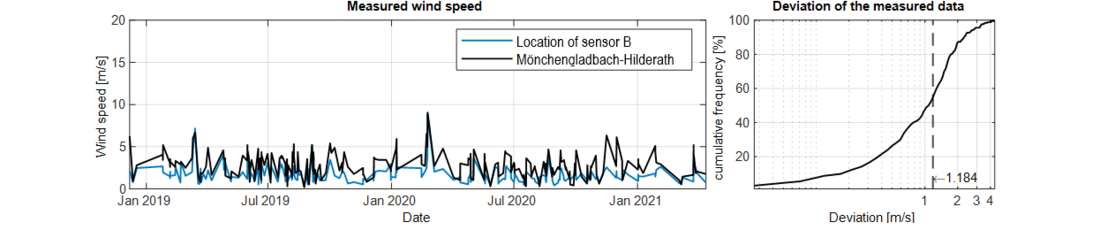
Figure 20 - Comparison of the measured annual extreme values of the 10 minutes mean wind speed for sector 9 (deviation: 90 % < 2.3 m/s)
As expected, the values for the wind speeds in Mönchengladbach-Hilderath as well as of sensor B increase. However, not to the same extent, consequently an approximation of both measurement series takes place. The deviations of the two data series in Figure 21 are now 90 % smaller than 2.2 m/s.

Figure 21 - Comparison of the homogenised annual extreme values of the 10 minutes mean wind speed for sector 9 (deviation: 90 % < 2.2 m/s)
3.3. Case study DWD station Balingen-Bronnhaupten
In the third case study, the weather parameters air temperature, precipitation, relative humidity, dew point temperature and wind speed are converted to the location of the DWD station Balingen- Bronnhaupten and compared with real measured values at the location.
3.3.1. Calculation of the weather parameters air temperature, precipitation, relative humidity and dew point temperature
Figure 22 shows the stations used and the distances to the pylon site. The data history covers a period from January 2018 to February 2022.
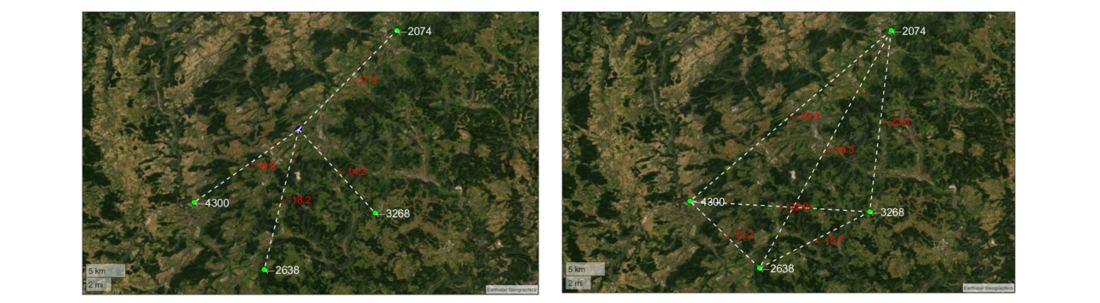
Figure 22 - Surroundings between the DWD stations Balingen-Bronnhaupten (blue dot) and Freudenstadt from Google Earth
For this calculation of the weather parameters, data on the Balingen-Bronnhaupten station location under consideration can be used from the following stations:
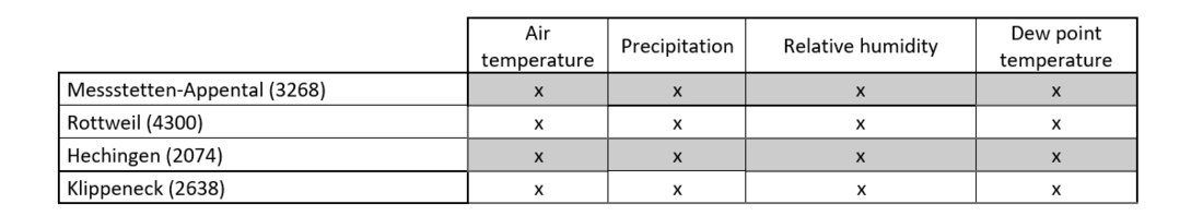
Table 12 - DWD stations for the calculation of weather parameters in Balingen-Bronnhaupten
The conversions of the weather parameters air temperature, precipitation, relative humidity and dew point temperature show similar deviations as in the first two case studies. The air temperature achieves a deviation of less than 1 K in 70 % of cases. The converted precipitation values show a deviation of less than 1 mm/h in 90 % of cases. The measurement of the relative humidity reaches 85 % of all values with an absolute deviation of 10 %. The conversion of the dew point temperature, as with the air temperature, achieves a deviation of less than 1 K in 75 % of cases.

Figure 23 - Cumulated deviations of the real measured values and the synthetically generated values at the Balingen-Bronnhaupten site
In this third example, the two stations Freudenstadt and Balingen-Bronnhaupten are at different altitudes above sea level. The difference in altitude is 178 m. Based on an altitude-dependent correction factor of 0.0065 K/m, a temperature adjustment of 1.157 °C results.
3.3.2. Calculation of the weather parameter wind
To validate the procedure for converting wind speed under the influence of topography, two DWD weather stations were compared that are located at approximately the same altitude above sea level. The Freudenstadt station is located in an exposed position, the influence of which is clearly evident in the measured wind speed values. The Balingen-Bronnhaupten station is located on flat terrain and is therefore well suited for comparison. To illustrate the homogenisation procedure, the comparison is made here for sector 11. The remaining sectors show similar behaviour.
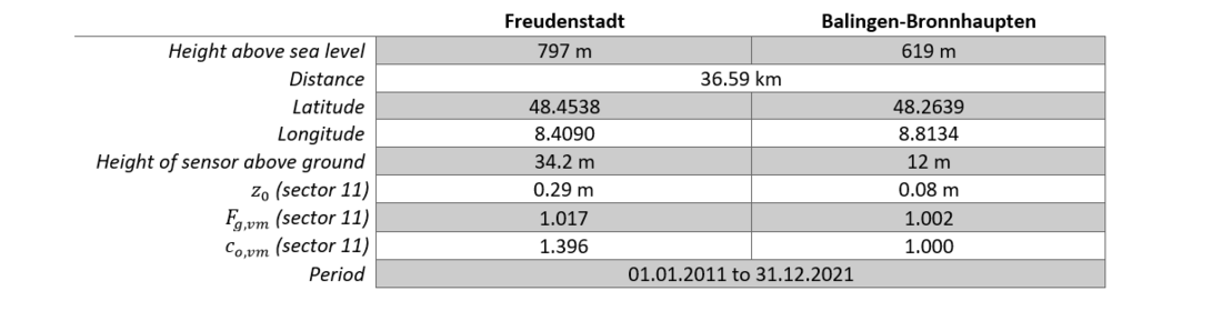
Table 13 - Data from the Freudenstadt and Balingen-Bronnhaupten weather stations
Both weather stations show a similar wind frequency, with wind speeds between 2 m/s and 5 m/s being the most frequent.
The annual extreme values of the 10 minutes mean wind speed of the two weather stations obtained by the conversion factor 1.06 differ, as expected, by less than 2.7 m/s for 90 % of the values. Both the roughness and the topography play a decisive role for this difference. Both aspects differ significantly between the sites. In addition, the values are influenced by the different positions of the measurement sensors above the ground. Since the topic of roughness is dealt with in the previous examples, the determination of the topography factor for the mean wind speed is explained below.
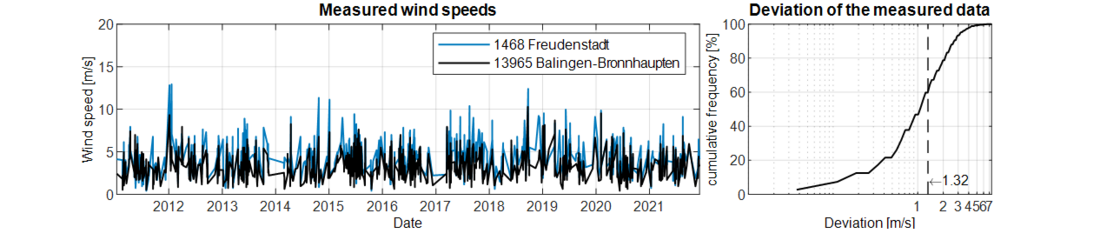
Figure 24 - Comparison of the measured annual extreme values of the 10 minutes mean wind speed for sector 11 (deviation: 90 % < 2.7 m/s)
The Freudenstadt weather station is located on the crest of an embankment. By simplifying the topography, the location can be defined as case 1 (see Chapter 2.2.7). As can be seen in the annual extreme values of the 10 minutes mean wind speed, the measured data experience an increase in comparison to the Balingen-Bronnhaupten station due to the exposed location. The topography coefficient is 1.396.
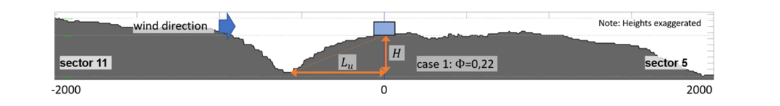
Figure 25 - Terrain topography in Freudenstadt
Data homogenisation is now used to create the regional wind climate model by applying the roughness coefficients and topography coefficients for data cleaning. The difference between the data is now 90 % of the values below 1.7 m/s and is considered negligible.

Figure 26 - Comparison of the homogenised annual extreme values of the 10 minutes mean wind speed for sector 11 (deviation: 90 % < 1.7 m/s)
4. Summary
For the probabilistic calculation proofs, extrapolation approaches were shown and explained within the scope of this paper. For the extrapolation of the weather parameters air temperature, global radiation, relative humidity, air pressure, precipitation and dew point temperature, the ordinary kriging approach used in the literature was applied. The extrapolation of the wind speed was calculated according to the approach of the standard [2] and [3], taking into account cadastral maps and height profiles. The methods were validated using three case studies and the corresponding absolute deviations were presented using cumulative frequencies. Extrapolation of the wind speeds to a site under consideration shows that 90 % of all values have a deviation smaller than 1.7 m/s - 2.2 m/s. Basically, it can be concluded that the mathematical approaches in the case studies have achieved good results, consequently they can provide good results for the probabilistic verification of the overhead line pylons as well as for the calculation of the current carrying capacity. It should be noted that the main focus of this paper is the determination of statistical distributions based on historical data sets, so that probabilistic calculations can be carried out on this basis. As shown in [10], this can be used, for example, for the static calculation of the failure probability for lattice towers. In [10], the distribution function of the wind speed on the side of the external forces was used and considered probabilistically with the resistance behaviour of the pylon.
Furthermore, it would be highly recommended to apply this method related to the application of the OHLs to the standardisation.
References
- VDE AR 4210-4.
- DIN EN 1991-1-4.
- DIN EN 1991-1-4/NA.
- ESDU 01008: Computer program for wind speeds and turbulence properties: flat or hilly sites in terrain with roughness changes, 2010.
- H. Wackernagel, “Multivariate Geostatistic”, Springer, Berlin 2003.
- ISO 4354: Wind actions on structures, 2009.
- "https://land.copernicus.eu/pan-european/corine-land-cover," [Online].
- United States Geological Survey: Shuttle Radar Topography Mission (SRTM), 2000.
- "https://cdc.dwd.de/portal/," [Online].
- S. Steevens, E. Ulloa Jimenez, N. Winkelmann, M. Mix, "Probabilistic safety concept in OHL construction", CIGRE, 2022.