Revolutionizing Energy: Smart Microgrids Driving down Costs and Carbon Foot Print Emissions through Advanced Spider Wasp optimization and BiGRU Techniques
Authors
Anirban MAITY, Atanu ROY - Dept. of Marine Engineering, The Neotia University (TNU), India
Sabyasachi PRAMANIK - Dept. of Computer Science and Engineering, Haldia Institute of Technology (HIT), India
Pulok PATTANAYAK - Dept. of Electrical Engineering, The Neotia University (TNU), India
Sajjan KUMAR - Dept. of Electrical & Electronics Engineering, SSN College of Engineering, India

Summary
MG (Microgrids) are increasingly recognized as a vital component in the transition to sustainable energy systems. Due to the emissions of particulate matter and substances, power plants face increasing regulatory scrutiny and this can complicate operations within MGs that strive for compliance with environmental standard, the operational cost of MGs includes fuel costs and battery degradation. To address the challenges associated with microgrids (MGs), various manual approaches have been explored. However, these manual methods reveal certain shortcomings, particularly in terms of performance efficiency. Hence, proposed study introduces enhanced SWO (Spider Wasp Optimization) algorithm, by incorporating proposed PPCBO (Preventing Premature Convergence Balanced Optimization) in the exploration phase and proposed FFSPM (Feature Filter Selection Point Measuring) technique in the exploitation phase of SWO algorithm. Proposed PPCBO mechanism adjust the exploration parameters dynamically, taking into account the diversity of current solutions. This adjustment modifies the search behavior to prevent clustering around local optima. Similarly, FFSPM function utilizes feature filter selection on a narrowed search space that includes only the most relevant features. This reduction enables the algorithm to concentrate its exploitation efforts on a smaller subset of features, thereby enhancing its ability to converge more quickly on optimal solutions. As a result, computational resources are used more efficiently, leading to rapid convergence process and much more enhanced solutions. Once the optimal features are extracted in feature optimization process, energy consumption and power usage of the grid is calculated using BiGRU (Bidirectional Gated Recurrent Unit) technique. Eventually, the proposed model focuses on minimizing the emission of carbon footprint by obtaining lower error rates of RMSE, MAE and MSE and remarkable CO2 reduction value.
Keywords
Microgrids, CO2 Emissions, Cost Reduction, Spider Wasp Optimization, Bidirectional Gated Recurrent Unit1. Introduction
MG’s (Microgrid) can utilize a diverse range of energy sources [1, 2], such as solar, wind, biomass, fuel cells and traditional generators [3, 4]. While fossil fuels have historically been the primary energy source for MGs, there is a growing trend towards adopting renewable energy options [5]. This shift is influenced by various factors, including the local availability of renewable resources, fuel costs and the reliability of the main grid. However, due to the inherent unpredictability and intermittency of RES (Renewable Energy Sources), energy storage systems are essential for ensuring a stable and dependable electricity supply [6] . These systems enable MGs to capture surplus energy produced during low demand periods and release it during times of high demand or when renewable generation falls short. Moreover, MGs are increasingly recognized for its role in minimizing energy emissions and costs while enhancing energy resilience [7]. By integrating RES, MGs can significantly lower carbon emissions and improve the overall energy efficiency [8]. It provides localized power generation, which minimizes the transmission losses and allows for better control over energy costs. Figure 1 shows the total renewable power capacity and expected capacity for net zero.
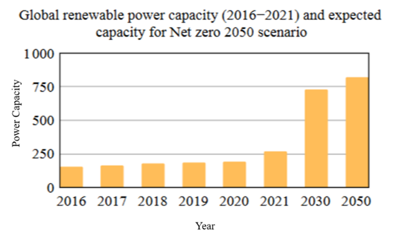
Figure 1 - Total Renewable power capacity and expected capacity for Net zero [9]
Hence, in order to detect the process efficiently, various traditional models such as energy sector equilibrium models, BCA (Benefit Cost Assessment) models, model predictive control and mixed-integer linear programming have been explored. Hence, the MPC (Model Predictive Control) model [10] has been used in the study for optimizing the carbon emission and economic costs.
However, these models are known to be extremely time-consuming, computational complexity as MPC unravels complex optimization problems at each control step, which can be computationally intensive. Moreover, manual methods are known to be sensitive, thus any discrepancies between the actual system behavior and the model assumptions can lead to suboptimal control actions, resulting in poor performance in terms of stability and efficiency. Besides, manual approaches lack in flexibility in adapting to rapidly changing conditions and unexpected disturbances. Hence, to tackle these issues, AI-based algorithms are preferred. AI algorithms are used because they can optimize the operation of the hybrid systems that combine diesel generator with RES, such as solar and wind [11, 12]. As RES are inherently intermittent, AI models play a crucial role in stabilizing the grid. Some of the common AI-based optimization algorithms used include the WOA (Wolf Optimization Algorithm) [13] technique which optimally schedules the distributed resources at minimum costs and emissions. Likewise, the adaptive GA (Genetic Algorithm) [14] has been used for optimizing the microgrid usage and leading to considerable cost reduction in performance. Similarly, the multi-objective GA algorithm [15] has used for scheduling the production and consumption of greenhouse gases. Besides, sine-cosine algorithm has been deployed along with the crow search algorithm and grey wolf optimizer for estimating the generation costs and emissions in the MG.
Though there are various existing works used for the reduction of costs and emissions from MGs and predicting energy consumption, there exist a few drawbacks of state-of-the-art approaches which includes, higher error rates of the model, vanishing gradient issue, limited scalability, slow convergence rate, computational resource intensity, overfitting of the existing models, complexity of the models as advanced predictive models can make it overly complex, making it difficult to employ. Therefore, in order to address the challenges, proposed model opts for SWO (Spider Wasp Optimization) algorithm, by utilizing PPCBO (Preventing Premature Convergence Balanced Optimization) in the exploration phase, where PPCBO mechanism dynamically adjust the exploration parameters based on the diversity of the current solutions and modify its search behavior to avoid clustering around local optima. This permits the algorithm to uphold a balance between exploring new areas of the solution space and exploitation known good solutions. Likewise, FFSPM (Feature Filter Selection Point Measuring) Technique used in the exploitation phase. By applying the feature filter selection, the proposed SWO algorithm narrows down the search space to only features that are most relevant. This reduction allows the algorithm to focus its exploitation efforts on smaller subset of features, enhancing its ability to converge on optimal solutions more quickly. As a result, computational resources are utilized more efficiently, leading to faster convergence times and improved solution quality. After utilizing the enhanced SWO for feature optimization, the BiGRU (Bidirectional Gated Recurrent Unit) model is used for predicting energy consumption and power usage by the MGs. Eventually, the performance of the model is gauged using various metrics such as MSE, MAE, RMSE and R2 and emphasize the significance of the proposed model in reducing the carbon foot print from power plants.
1.1. Research Objectives
The major research objectives of the proposed work is listed as follows,
- To minimize the operational costs such as fuel costs and battery degradation and reduce carbon foot print (CO2) from power plant generators by selecting the optimal features for the MG using proposed enhanced SWO algorithm.
- To integrate PPCBO (Preventing Premature Convergence Balanced Optimization) in the exploration phase and FFSPMT (Feature Filter Selection Point Measuring Technique) in the exploitation phase in the proposed SWO.
- To predict the energy consumption and power usage of the MG using Bidirectional Gated Recurrent Unit model.
- To evaluate proposed model efficiency by using error metrics such as MSE, MAE, RMSE and CO2 reduction value than existing model.
The paper is organized in the following way. In section 2, review of the existing works done by various researchers are incorporated. Section 3 focuses on implementing the proposed feature optimization algorithm and prediction based BiGRU model for the proposed work. Section 4 focuses on obtaining the results attained using proposed algorithms, where various graphs such as actual vs. predicted plots, box plots, and histograms. Besides, the model is evaluated using different metrics for assessing the performance of the model. Eventually, section 5 summarizes the entire work along with future recommendation.
2. Literature Review
Managing cost in MG poses a considerable challenge, primarily because the energy produced often comes from a mix of renewable and non-renewable sources [16]. Therefore, improved ARO (Artificial Rabbit Optimization) algorithm [17] was employed for optimizing the cost of operation based on current load demand, prices of energy and generation capacities. Findings of the study has showcased that, improved ARO algorithm has delivered better outcome than ARO algorithm. Conversely, the prior study [18] was developed a nature-inspired algorithm, Spider Wasp Optimization (SWO), based on female spider wasp behaviors, offering unique strategies for diverse optimization problems. It was validated against nine other metaheuristics using four benchmarks such as standard functions, CEC2017, CEC2020, and CEC2014, demonstrating superior performance. SWO also proved effective in real-world engineering design and photovoltaic model parameter estimation problems. Another study [19] presented a Multi-strategy Improved SWO (MISWO) algorithm enhances the traditional SWO by incorporating the Grey Wolf Algorithm for better initialization, adaptive step size and Gaussian mutation for improved search, dynamic Trade-off Rate (TR) selection, and dynamic lens imaging reverse learning to escape local optima. This approach was validated through tests on benchmark functions and engineering problems, showcasing its superiority over other algorithms. Notably, the author in [20] introduced a feature selection method referred as FSSWO, for software fault prediction, addressing challenges like high computational complexity and poor generalization in existing approaches.
Similarly, cost function of the MG has been reduced using MLP-ANN (Multilayer Perceptron- Artificial Neural Network) and GA [21]. Though the model has focused on cost reduction in MG, the future work of the study emphasizes on green-house gas emission using prediction strategy of PV power and optimal ESS (Energy Storage System) implementation in the test MG. Integration of solar MG and wind MG [22] has considered in the study for dynamic power flow management with the aim to enhance the quality of power and for reducing the burden of the grid. Besides, MG has designed with high renewable fraction, low electricity cost and low emission [23] by integrating RES such as PV, FC, battery and Diesel generator. Simulation and performance evaluation revealed that the suggested RES delivered optimal outcomes with 73% of the total energy generated by PV panels, 3% from DG and 24% from fuel cells. Emissions pose serious threats to the environment, underscoring the critical importance of implementing strategies to minimize them. Hence, a hybrid neural network model [5] has employed for predicting different emissions from the gas turbines such as CO (Carbon Monoxide) and NOx (Nitrogen Oxide). The hybrid model combined CNN and BiLSTM with modified extrinsic attention regression model. Therefore, findings of the model has deliberated in enhanced GT functioning and reduced emissions. Likewise, ML algorithms such as ANN, SVM and DL [24] were used for forecasting the gas emission prediction. Findings of the work has stated that, gas emission has increased at high rate and it is important to employ more advanced models overcome these limitations. The author in [25] has explored AttiBiGRU (Attentional-BiGRU) prediction model for effective feature extraction and an improved Arithmetic Optimization Algorithm (CGAOA) for optimal hyper tuning and demonstrated satisfied level of accuracy. Similarly, the author in [26] has combined AttiBiGRU with GGBERO (Greylag Goose Optimization and Al-Biruni Earth Radius), to address the challenges of predicting CO2 emissions due to their non-linear and temporal nature.
Besides, it is crucial to track the rate of gas emissions generated during power production in order to adhere to industry standards for emission control [27]. Therefore, a stacked ensemble ML [28] based predictive model has deployed for CO and NOx emissions. Hence, the simulation outcomes indicated that the use of SEM achieved remarkable reduction in RMSE, decreasing NOx emissions by 5.7% to 93.8% and CO emissions by 1% to 41.5%, when compared to other ML techniques. The advancement and adoption of RES have garnered significant societal interest in response to environmental challenges. The relatively low environmental impact of clean energy, derived from renewable power sources, is viewed as a highly effective solution to these pressing issues. Hence, the lightning search algorithm [29] has been used for EMS of MG to limit the overheads of the electricity generation and to decrease the carbon dioxide emission from the MG. Results of the study has revealed that, efficacy of the method has outperformed other procedures in terms of least total operating cost of distributed energy resources. Correspondingly, the study [30] has focused on developing a predicate model for transient NOx emission in hydrogen diesel engines by employing ML techniques. Correspondingly, a hybrid setup has been used in the study, which consisted to of BESS, DG and PHS [31] for enhancing the energy management system, minimizing the operation costs and also to reduce the carbon emissions. In order to achieve this, SDDP (Stochastic dual dynamic programming) has been taken. The findings of the work has stated that, SDDP reduced the costs and promote sustainable energy solutions in the evolving energy landscape.
The primary objective of the paper [32] has focused on reducing the total greenhouse gas emission such as CO, SO2, NOx, CO2 by diesel generators, by integrating the PV sources. This approach takes into account the typical power profiles and consumption patterns in Colombia by using ANN algorithm. The numerical analyzes of the model has indicated that the implementation of these PV sources can lead to a reduction in gas emissions ranging from 17% to 19%, depending on the quantity and size of the installed PV systems. Similarly, reducing the overall operational costs [33] associated with energy generate and consumption and minimizing the environmental impact by lowering emissions produced by diesel generators and other components of the MG. Optimization process has been carried out by using GA (Genetic Algorithm) and MATLAB Simulink [33]. Experimental outcome of the study has showcased that, the model optimization model reduce the total cost by 3.5% and carbon emission of 0.7%. Likewise, the focus of the work has emphasized on evaluating the emissions of air pollutants from DG and explored the potential for reducing the emissions through the implementation of MGs and solar energy solutions. Therefore, the HOMER framework [34] has been utilized to design an optimized MG system that integrated DGs and solar PV. The optimized diesel based MG achieved a 19% reduction in specific fuel consumption and a 5% reduction in operational costs compared to the baseline setups.
DGs are extensively utilized in MG and off grid systems for rural electrification [35, 36]. The strategies for sizing and selecting these generators during the planning phase of MGs are critical for optimizing cost efficiency and minimizing the environmental impacts. Hence, LMIP (Linear Mixed Integer Problem) model [37] has been implemented and this model minimizes the cash flow expenses by choosing ideal size and no. of DGs for reducing the fuel consumption. Similarly, MOSSA (Multi-Objective Salp Swarm Algorithm) [38] has been used to ensure that the system works better on RES. Analytical outcome has demonstrated that MOSSA has delivered considerable performance for obtaining ideal design solutions. Contrastingly, AI based MLP and SVR [39] are used for forecasting the emission of CO2. Result of the model has stated that, PV and battery system, supplemented by a limited amount of DG as a backup power source, represents the most effective combination for all scenarios. DL based LSTM model [40] has employed in the model for forecasting the cost and to reduce the carbon emissions. The results exposed that around 29.4% of carbon emission cost has been reduced.
2.1. Problem Identification
Core concerns detected from the SOTA models is listed as follows,
- The limitations of [29] include the need for more efficient and intelligent optimization algorithms to enhance the management of Distributed Energy Resources (DERs) in Microgrid (MG) systems, improving cost efficiency, CO2 reduction and system stability.
- The study [28] lacks a comprehensive comparison across multiple metrics such as MAE, R-squared (R²), which are crucial for assessing the robustness and generalizability of the predictive model.
- There is a need for more robust forecasting techniques and scalable ESS models to improve the efficiency and resilience of hybrid energy systems at larger scales [40].
3. Proposed Methodology
3.1. Proposed Design
Proposed designs aimed at reducing both costs and emissions through optimized operational decisions are detailed in the following section. This comprehensive framework illustrates the mechanism employed in this research, which utilizes advanced feature optimization techniques alongside regression models. The objective is to enhance the operational efficiency while simultaneously addressing emission challenges. Hence, by leveraging feature optimization, key variables are identified that significantly influence both cost and emission metrics. The main objectives of the proposed work focus on,
- To minimize the operating cost
- To reduce the CO2 emissions and practice of fuel by ensuring the optimal usage of RES
- To effectively store or discharge energy from battery by using SWO for deciding when to charge the battery using RES.
Therefore, overview of the proposed framework is demonstrated in figure 2.
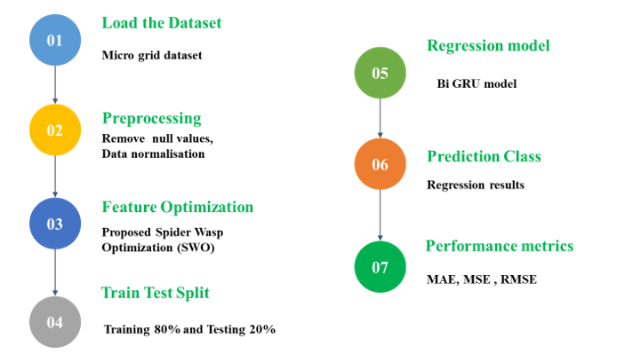
Figure 2 - Illustrates Steps involved in the Proposed Model
Figure 2 demonstrates the process involved in proposed framework, where the microgrid dataset is used. Once the dataset is loaded, pre-processing takes place, where removal of null values and data normalization is carried out. After pre-processing, feature optimization is carried out using the proposed SWO algorithm, where PPCBO and FFSPM are used in the exploration and exploitation phase. Using the proposed SWO, optimal features are selected for the model. After feature optimization, a train-test split is carried out, where the training data is split into 80% and testing data is split into 20%. Eventually, the regression model is used for predicting the energy consumption and usage of power of the model by using BiGRU approach. Finally, the performance of the model is assessed by employing metrics such as MAE, MSE, RMSE and R2.
Dataset Description
The simulation of a hybrid AC-DC micro-grid for the Payra area in Bangladesh uses solar, wind and natural gas as energy sources which includes seven data files, with the first being the original load demand and the others representing varied load scenarios (10%, 5% and 2.5% more or less). Each file contains 8761 instances, with 14 data columns including power outputs, fuel consumption, renewable energy penetration and battery charge/discharge information. The dataset represents various load demand scenarios for both AC and DC consumers. The input and output features include: Time, Photovoltaic panel Power Output (kW), Wind Turbine Power Output (kW), Generator Power Output (kW), Generator Fuel Consumption (m-3), Total Electrical Load Served (kW), Renewable Penetration (%), Excess Electrical Production (kW), Total Renewable Power Output (kW), Inverter Power Output (kW), Rectifier Power Output (kW), Battery Discharge Power (kW), Battery State of Charge (%). Power is formulated as: “Total Electrical Load Served (kW)'+'Battery Discharge Power (kW)”.
3.2. Feature Optimization- Proposed Spider Wasp algorithm (Enhanced SWO)
Feature optimization refers to the process of selecting the most relevant features from the data to improve the performance of the model and eliminate redundant data that impacts the accuracy and efficiency of the model. Though there are various algorithms for feature optimization, the propose model opts for the SWO algorithm as it is inspired by the behavior of spider wasps, which exhibit the complex searching and nesting behaviors. This biological basis allows the algorithm to mimic natural process effectively. Besides, the SWO reflects a unique balance between exploration strategy and exploitation strategy. This balance helps in avoiding local optima, thereby allowing the algorithm to explore a wider solution space effectively. Further, SWO employs guidance strategy like dual-median-point guidance, which improve the algorithms’ ability to navigate complex landscapes and escape local minima. Owing to these factors, SWO is preferred over algorithms for feature optimization.
The enhanced SWO algorithm starts by initializing the population. Following this, the positions of individual wasps are updated based on various behaviors such as searching, following, escaping, nesting and mating. This cycle continues until the optimization concludes, which occurs when a specified termination condition is met. The mathematical representation of these behaviors within the SWO optimization framework is outlined as follows.
a) Initializing the Population
Each spider wasp (female) signifies a solution to the problem to be so demonstrated using equation 1,
(1)
Here, yi is signifies the value of individual in the ith dimension and the variable D represents the scale or extent of the problem that needs to be addressed. When addressing optimization problems, it is often essential to create initial individuals within the specified boundaries of the problem, as indicated by equation 2.
(2)
Where, the variable r signifies the D dimensional random vector in the interval [0,1] , LB and UB highlights the upper bound and lower bound of the problem both of which are a D dimensional vector. SPWOi represents the data associated with the ith female individual. The N individuals are then organized into an initial population to facilitate the subsequent iterative optimization process, as represented by equation 3,
(3)
b) Searching Behaviour
During the searching phase, the female spider wasp arbitrarily navigates the population space with a fixed step size to locate suitable spiders for feeding her larvae, as described by equation 4,
(4)
In which, no. of iterations is denoted as t and represents the information of the ith individual at the t iteration.
and
represents two distinct arbitrary individuals within the population. Meanwhile,
signifies the new state produced by the ith individual following the search phase. The parameter µ1 is utilized to establish the search direction and is defined by the equation 5,
(5)
Where, a random number that follows the normal distribution is depicted as rn, while r1 is denoted as an arbitrary number within the range of [0, 1]. Furthermore, since the female spider wasp occasionally loses sight of the spider that drops from the sphere, the female spider explores the vicinity around the point where the spider has fallen, as indicated by equation 6.
(6)
In which, µ2 highlights the search direction and is demonstrated as the arbitrary individual in the population as heighted in equation 7.
(7)
Where, using equation 8, B is represented as,
(8)
In equation 8, random number generated within the interval [-2,-1] is represented as l and the search phase is formulated through equation, with equation 4 and equation 6 working in conjunction for detecting favourable region.
(9)
Where, both r2 and r3 is represented as the numbers in the interval [0,1] in equation 9.
c) Following and escaping behaviours
Once the female spider wasp has identified the location of its prey, it proceeds to hunt it. This hunting behaviour is represented in equation 10,
(10)
Here, ConFac showcases the distance control, which diminishes linearly from 2 to 0, as outlined in equation 11,
(11)
From Equation, it is detected that t and tmax showcases present no. of iterations and maximum no. of iterations. At the same time, the prey attempts to flee when it is under attack, and this behaviour is represented by equation 12,
(12)
Here, D dimensional vector is depicted as vec as stated by the normal distribution in the interval, [k,k] and k is demonstrated in the equation 13,
(13)
The resulting trade-offs between fleeing and hunting behaviours, achieved through randomization, are illustrated in equation 14,
(14)
During the process of optimization, the initial step involves using the searching behaviour to pinpoint areas that may hold the globally optimal solution. Subsequently, the algorithm incorporates following and escaping behaviours to prevent entrapment in local optima. Consequently, equation 15 is utilized to achieve a balance between these 2 behavioural strategies.
(15)
d) Nesting Behaviour
At this point, the female spider wasp captures the spider and brings it into a nest that has been previously prepared. Because the female spider wasp utilizes various besting techniques, two of these methods are taken into account in the SWO algorithm. The first method involves drawing the spider toward the area that is most advantageous for the female spider wasp, as illustrated in the equation 16.
(16)
Here, ideal individual in the population is depicted as PC* and the second method entails randomly selecting a female spider wasp from the population and establishing nests based on that individual’s location, as demonstrated in equation 17.
(17)
In equation 17, U is denoted as the binary vector and y is depicted as random number generated by levy flight and is depicted in equation 18.
(18)
In equation 18, 2 D dimensional random vectors in the interval [0, 1] is detected as r4 and r5 and the 2 nesting methods described above are evaluated based on the criteria outlined in equation 19,
(19)
Ultimately, the searching behaviour, along with the following, escaping and nesting behaviours, is assessed using equation 20,
(20)
e) Mating Behaviour
At this stage, the mating behaviour of the female spider wasp is primarily emphasized in this phase to facilitate the creation of a new spider wasp, as described by equation 21,
(21)
Where, crossover operation between the solutions of is denoted as crossover with the probability of crossover as CR. Here, the value of CR is assigned as 0.2. Further,
is represented as female spider wasp and
is denoted as male spider wasp and eventually, the male spider generation is depicted in equation 22 as
(22)
Here, random number produced in relation to normal distribution is illustrated as . Likewise, exponential constant is depicted as e.
(23)
(24)
Where, the value of the objective function in equation 23 and 24 is associated with the individual is represented by f(X). In conclusion, the TR (Trade-off) rate assesses the balance between hunting, nesting and mating behaviours.
f) Population Reduction and Memory Optimization
Upon completion of the mating behaviour, the population of female spider wasp will be optimized, leading to improved outcomes and a more rapid convergence in the optimization process. The mathematical process is depicted in equation 25 as
(25)
Here, minimum size of population is denoted as Nmin and it is utilized during the process of optimization for avoiding the spider wasp algorithm into the trap of local optimum. Eventually, the newly updated individuals are evaluated against those from the previous generation.
3.2.1. Proposed SWO algorithm with emission and cost
Though the existing spider wasp optimization algorithm has delivered considerable performance in selecting the optimal features for the model, there exist a few limitations that need to be addressed. Some of the common limitations identified are weak exploitation capability and low population diversity. Additionally, the model is susceptible to becoming trapped in local optima, making it difficult to find the true shortest, collision-free path within the given time constraints. Furthermore, the inability to detect a global optimum solution, which is crucial for effectively minimizing costs and emissions in complex microgrid environment is considered as one of the drawbacks of the model. The convergence rate of traditional SWO can be slow, specifically in high dimensional search spaces. This inefficiency can lead to longer computation times and less timely solutions. In some cases, traditional SWO can potentially struggle with balancing exploration and exploitation. An inadequate balance can result in either premature convergence or excessive searching without meaningful progress. These drawbacks suggest that while SWO has potential, its traditional form may require enhancements to effectively tackle the specific challenges associated with optimizing microgrid systems. Therefore, to tackle these limitations, the proposed model utilizes a prevention premature convergence balanced optimization in the exploration phase and feature filter selection point measuring technique in the exploitation phase. Figure 3 showcases the proposed SWO process.
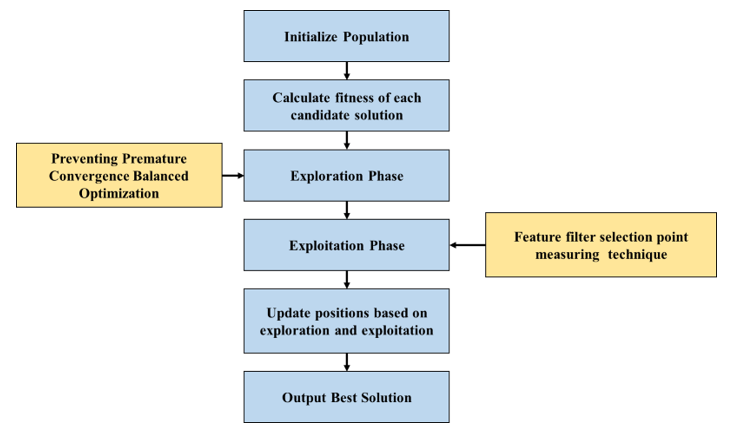
Figure 3 - Proposed SWO process
Similar to traditional SWO, the proposed model starts by population initialization. Hence, to initialize the population for proposed SWO algorithm, first, define the lower and upper bounds of the variable bounds. Then, a LHS (Latin Hypercube Sampling) method is employed for generating a population of candidate solutions, where the number of sample corresponds to the number of agents. This population is scaled by the difference between the upper and lower bounds and shifted by the lower bounds to ensure that all candidate solutions fall within the defined limits. Subsequently, the fitness of each candidate solution is calculated by evaluating the generator output and battery charge power; specifically, emission are determined by multiplying the generator output by 0.267, while the total cost is computed as the sum of the product of the generator output and 0.5 plus the emission. After generating fitness of each candidate solution, exploration phase undergoes. Where PPCBO (Preventing Premature Convergence Balanced Optimization) is used for addressing the weak global search ability of SWO. PPCBO approach integrates the dynamics of learning factors with the varied information gaps among individuals to improve population diversity during the algorithm’s solving process. Thereby enhancing the global search performance of SWO. In exploitation phase, FFSPM (Feature Filter Selection Point Measuring Technique) technique is used. In this framework, individuals gain insights from a group of peers rather than solely relying on their own experiences. This not only improves their individual performance in exploiting available resources but also maintains diversity within the group, leading to a more effective balance between global exploration and local exploitation phases. Further, proposed FFSPM is added to the nesting behaviour of proposed SWO for enhancing the ability of the algorithm for escaping the local optimal trap. After iterating through the defined number of generations, optimal solution is identified.
Thus, the mathematical equations for the proposed work is defined as follows,
(26)
(27)
Here, gap between the better and best individual is depicted in the equation 26 and 27. Likewise, learnability degree for each set of disparities is assessed using the equation 28.
(28)
In equation 28, LAi is defined as the learning ability of ith individual and objfmax is represented as the objective function.
(29)
(30)
Here, the equation 29 and equation 30 showcases that the model can commendably boost the algorithm diversity and thus enhance the performance of the algorithm. Further, to enhance the exploitation capability as much as possible while sustaining high exploration performance, FFSPM is used.
(31)
Where in equation 31, the co-efficient C minimizes from 0 to 2 as the no. of. Iterations maximizes, which enables that the bootstrapping needs to be reinforced in the pre-iteration period and then it is diminished gradually in the later part of the iteration phase for ensuing that the algorithm converges precisely. Eventually, bootstrapping is denoted as and it is expressed in the equation 32,
(32)
(33)
Here, represents the better individuals in the iteration and this is sorted based on the value of the objective function. Bootstrapping via FFSPM enhanced the algorithm’s convergence rate while also increasing its capacity to escape local optima. Besides, in equation 33 describes the update mechanism for a variable
at time t+1 based on its previous values, SPWObetter at time t. Further, cos(2πl) term introduces a periodic modulation, where l can be interpreted as a parameter that influences the degree of adjustment based on a cosine function, oscillating between -1 and 1.
Hence, the process showcases the algorithm’s capability to escape local optima in solving the path planning challenge, thereby strengthening its ability to seek global optimal solutions.
(34)
In equation 34, γ is showcased as the scale factor, SPWO represents the solution, path length is signified asMN. Likewise, D is characterized as the average distance from the intercalated points along the path to all hindrances. Therefore, proposed spider wasp optimization algorithm aids in minimizing the operational costs and finds the optimal times to the rung the power plant generators, thereby reducing the fuel use and emissions by relying on cleaner energy sources when possible.
3.3. Regression using Bidirectional Gated Recurrent Unit (BiGRU)
Once better features are identified using the proposed SWO by helping the microgrid to minimize both costs and energy emissions, power usage and energy consumption of the model is predicted using the BiGRU model. Thus, in order to accomplish this process, the proposed model opts for BiGRU model. Though there are various models which can be used for usage of power and energy consumption, the proposed work utilizes BiGRU model since, the BiGRU model processes data in both forward and backward directions, allowing it to capture dependencies from both past and future time stamps. This is very much helpful and beneficial in energy consumption forecasting, where patterns typically do not depend on historical data and other data patterns. Besides, the BiGRU model are designed to handle long sequences of data effectively. This capability is important for precisely modelling the complex temporal dynamics of energy usage, which is influenced by different factors over extended periods. Compared to other networks, BiGRUs have fewer parameters due to its simple gatting mechanism which can result in faster training times and reduced computational overhead. This efficiency is advantageous when processing huge datasets typical in energy consumption forecasting. Therefore, the overall capability of the BiGRU model to effectively learn from sequential data, coupled with its integration capabilities and computational efficiency makes it as a preferred choice for predicting power usage and energy consumption in microgrids.
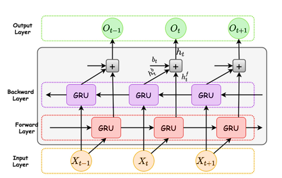
Figure 4 - Architecture of BiGRU model [41]
The overall functionality of BiGRU model is depicted in Figure 4. The bidirectional nature of the BiGRU model enables it to utilize information from both ends of a sequence, which is especially advantageous in predicting power and energy consumption. the fundamental architecture of a BiGRU consist of one or more BiGRU layers that process input sequences in both forward and backward directions, allowing for the capture of contextual information from both sides. Each BiGRU layer comprises a forward layer and a backward layer (reverse layer). The forward layer sequentially analyses the input data from beginning to end, effectively identifying relationships between the current input and all preceding inputs. Conversely, the backward layer processes the input in reverse order, from end to start, which allows it to recognize dependencies between the current input and subsequent inputs as perceived through forward processing. This dual approach enhances the model’s ability to understand complex temporal dependencies within the data.
The input layer receives a sequence of data X=[x1,x2, ... . xT]s, where T is defined as the length of the sequence and each input xt is denoted as the vector of features. The hidden state at time step t is computed using the formula in equation 35,
(35)
Where, hdt denotes the hidden state at time t. zt is denoted as the update gate, controlling how much of the previosu hidden state to keep and is the candidate hidden state, which is generated based on the current input and the preceding hidden state.
For update gate calculation, the mathematical expression used to describe this process is denoted in the equation 36,
(36)
Where, σ is denoted as the sigmoid activation function, wei is estimated as the weight matrix for the update gate and xi is considered as the input at time t. Eventually, the candidate hidden state is estimated and demonstrated in equation 37,
(37)
Here, Weih is denoted as the weight matrix for the candidate hidden matrix. Hence, the final output is derived from the combined of the forward and backward passes. This involves taking the last hidden state from the both directions or applying layers for producing the final predictions.
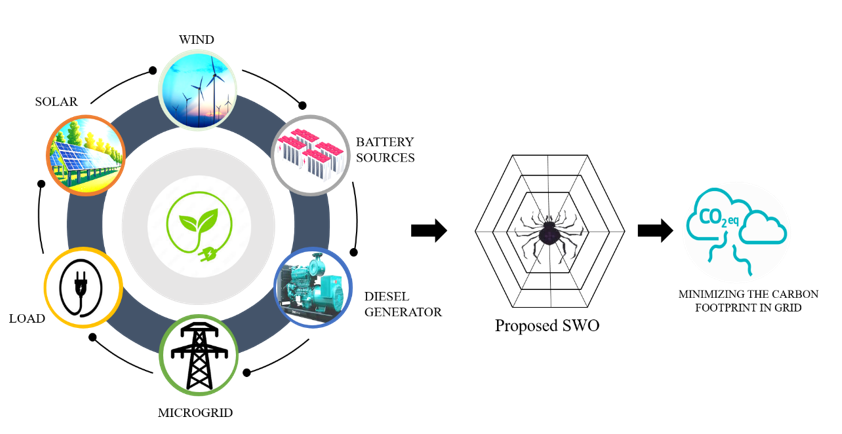
Figure 5 - Model Architecture of the Proposed Model
Figure 5 depicts the model architecture of the proposed model which involves the microgrids, battery sources, wind, solar, load and diesel generator which is led into the proposed SWO for minimizing the carbon footprint in the grid. The prosed study is employed BiGRU over other model LSTM,GRU for microgrid energy prediction was based on its ability to capture comprehensive bidirectional temporal dependencies, which is crucial as energy patterns are influenced by both past and future events. BiGRU also offers an efficiency advantage over LSTM and BiLSTM due to its simplified gating mechanism, resulting in faster training and fewer parameters without significant accuracy loss, a vital aspect for real-time applications. Additionally, BiGRU exhibits robustness in modeling long sequences, mitigating vanishing gradients and generalizing well even with potentially noisy historical data. Finally, its suitability for sequential data, compared to CNNs which excel at local pattern extraction but struggle with long-range dependencies, and its complementary nature with the SWO-optimized feature set, which provides high-signal input, allowing it to model the refined temporal patterns more effectively.
3.4. Internal Assessments
Apart from BiGRU, present research also uses algorithms like SVM, decision tree and random forest for predicting the power usage and energy consumption of the model.
a) SVR
SVR is one of the approaches opted by the present research for prediction mechanism. The key idea behind SVR is to detect a function that deviates from the actual target values by a value no greater than a specified margin. This mechanism uses a subset of the training data called support vectors, which are the data points closest to the decision boundary. The SVR algorithm aims to minimize the error while maintaining a flat function, which is accomplished through the use of a loss function that penalizes deviations from the margin. The flexibility of SVM allows it to handle both linear and non-linear relationships by employing kernel functions, which transform the input space into higher dimensions where linear regression can be applied effectively. The algorithm for SVM is depicted.
| Algorithm I : Support Vector Regression |
|---|
Input: Training data (X,y), where X is the feature set and y is the target variable |
b) Decision tree
Decision tree operates by recursively splitting the data into subsets based on feature values to create a tree-like model. Each internal node represents a decision based on an attribute, while leaf nodes represents the predicted output. For regression part, DT uses criteria like MSE for evaluating splits and the process begins at the root node with the entire dataset and continues until stopping criteria are met, such as achieving a maximum depth to minimum number of samples in a node. The final prediction for new data points is made by traversing the tree to the appropriate leaf node and generates its average value. This approach is intuitive and interpretable but at some cases, it can result in overfitting of the model. Algorithm II denotes the DT process.
| Algorithm II : Decision Tree |
Start |
c) Random forest
| Algorithm III : Random Forest |
Input preparation: Start with a training set S that includes features F and a specified number of trees n. |
Consequently, algorithm such as DT, SVR and RF are widely employed in the predictive modeling process. Each of these algorithm offers unique strengths and methodologies for performing prediction tasks. The outcomes generated by these algorithms will be presented and analyzed in the following section, providing insights into their performance and effectiveness in the MG setup.
4. Results and Discussion
Results obtained using proposed method is demonstrated in the present section, where exploratory data analysis, performance analysis and comparative analysis are deliberated numerically to reflect the effective performance of the proposed model when compared to other models.
4.1. Performance Metrics
Four metrics are considered for assessing the performance of the model, which includes RMSE, MSE and MAE.
a) RMSE
It is used to calculate the average variance amongst values in the classification and actual values.
(38)
b) MSE
It is used to measure the average squared difference between predicted and actual values.
(39)
c) MAE
It is signified as the average of the absolute dissimilarity between predicted and actual values.
(40)
d) R² Metric
It is the proportion of variance in the dependent variable that is predictable from the independent variables.
(41)
4.2. Explanatory Data Analysis (EDA)
EDA is a fundamental process that involves analyzing and visualizing the datasets to uncover its key characteristics, detect patterns and explore relationships between variables. Hence, EDA of the proposed study is demonstrated in the consequent section.
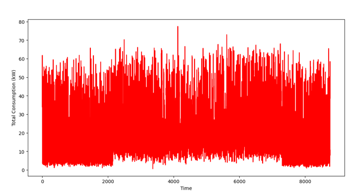
Figure 6 - Total consumption over Time
Figure 6 represents total power consumption (in kW) over a period of time. The x axis shows time, while the y axis shows he total consumption (kW). The power consumption is highly variable, ranging between 0 and 80 kW. The lower bound of consumption fluctuates mostly between 0 and 10 kW. Therefore, figure 6 shows a high and stable energy demand with transient peaks.
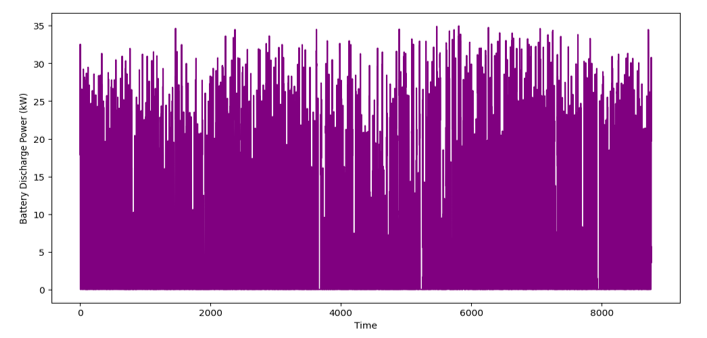
Figure 7 - Battery Discharge power over time
Figure 7 shows the power discharged from a battery system over time, measured in kW. The discharge power ranges from 0 kW to 35 kW. The pattern is highly variable, with frequent spikes and dips across the varied timeline. The values maintain a consistently high baseline, indicating that the battery is actively supplying significant power throughout.
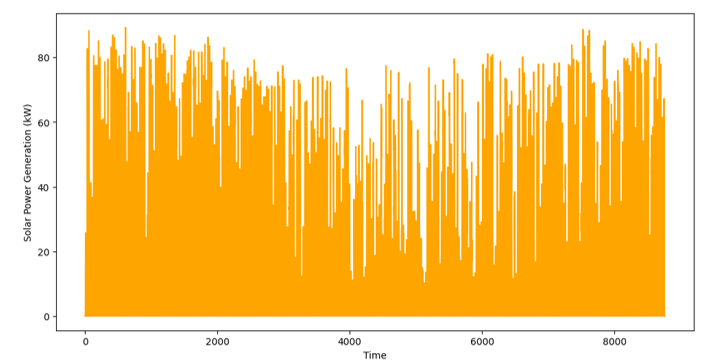
Figure 8 - Solar power generation over time
Likewise, figure 8 demonstrates the solar power generation over time, also measured in kW. Solar power generation fluctuates between 0 kW and approximately 80-90 kW. The pattern exhibits variability, with occasional sharp drops. A gradual increase in the output is noticeable around 6000-9000 time range, due to the solar conditions.
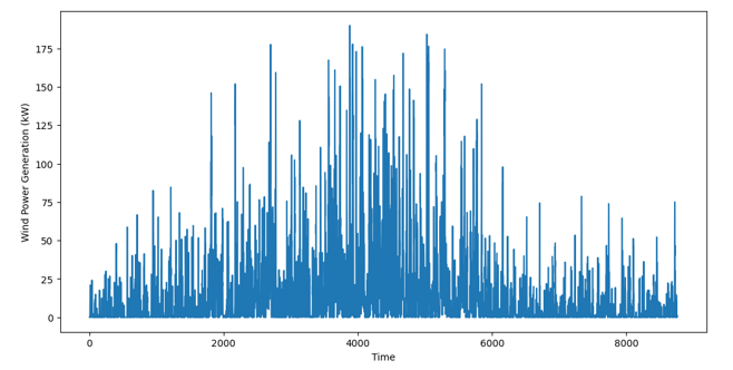
Figure 9 - Wind Power generation over time
Wind power generation over time, measured in kW is depicted in figure 9. Initially, wind power generation is minimal, often close to 0 kW. Between time steps 1000 s to 4000 s, the power generation gradually increases in amplitude with peak values exceeding 175 kW. This indicates a period of higher and more sustained wind speeds. Around the mid-point, the variability of wind power is at its highest. This implies period of rapid changes in wind conditions.
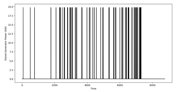
Figure 10 - Diesel Generator power over time
Diesel generator power over time is depicted in figure 10. Unlike the wind power graph or solar power graph, these diesel generator output is sporadic, with distinct bursts of power generation. The diesel generator remains at 0 kW for extended periods. When active, the diesel generator consistently outputs approximately 20 kW, indicating that it operates at a fixed capacity when needed. Around 4000 s to 6000 s, there is a higher frequency of DG activity. This correlates with the high variability in wind power during the same period and toward the 9000 s, DG usage decreases as wind power generation stabilizes at low levels. Therefore, it is reflected that, DG serves as a stabilizing source of power.
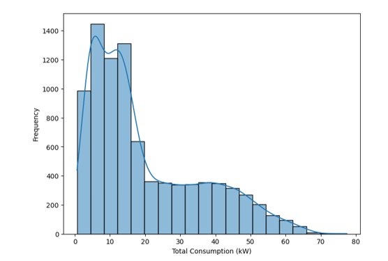
Figure 11 - Distribution of load
Distribution of load (histogram with density curve) is demonstrated in figure 11. The x axis shows the total consumption (kW) while the y-axis indicates the frequency. The overlaid density curve highlights the probability distribution. The distribution is right skewed, with a majority of consumption values concentrated at lower ranges and a long tail toward higher values. Consumption between 5-15 kW occurs most frequently, with the highest peak around 10 kW.
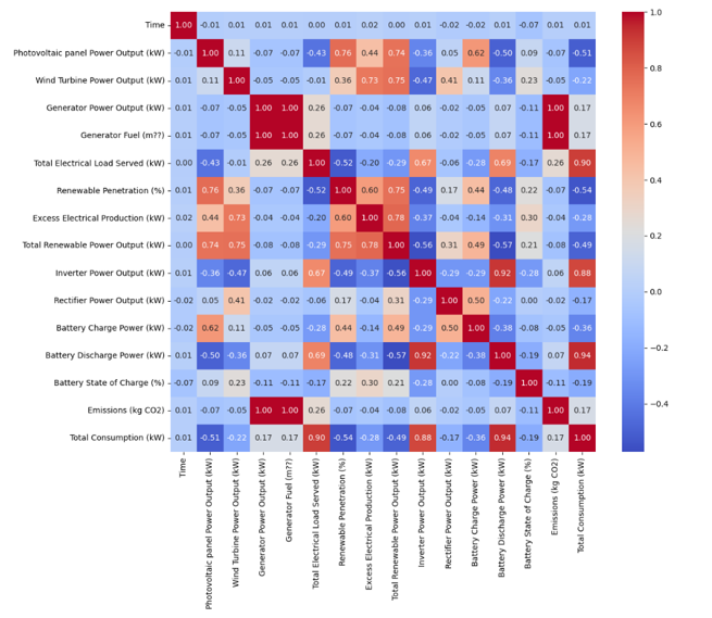
Figure 12 - Correlation Matrix
The Heatmap (correlation matrix) is demonstrated in the figure 12, where the heatmap shows the correlation coefficient between different variables related to energy production, consumption and system metrics. A correlation coefficient ranges from -1 to 1. Renewable penetration (%) and total renewable power output (0.78) shows that, High renewable energy output aligns strongly with greater renewable penetration. likewise, battery discharge power and total consumption (0.94) indicates that high consumption often requires significant battery discharge and inverter power output & total consumption (0.88) demonstrates that inverter’s output scales with total demand. Hence, it is illustrated that, battery systems play a huge role in balancing consumption and renewable energy production.
4.2. Performance Analysis
Performance of various traditional algorithms along with proposed algorithm is demonstrated in the performance analysis section, where figures like actual vs. predicted, box plot, histogram and other plots are covered in the section.
a) Decision Tree
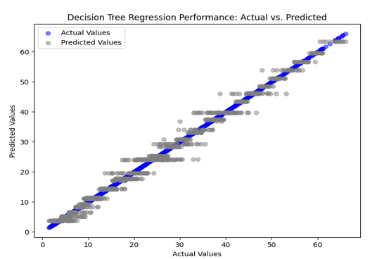
Figure 13 - Decision tree Regression performance: Actual vs Predicted
Figure 13 shows the regression performance of actual vs. predicted values obtained by DT. The points closely align the diagonal, indicating the predicted values match the actual values well for many data points. Besides, there has been no drastic deviations from the diagonal, indicating the absence of extreme errors in prediction. Hence, the model suggested the overall predictive accuracy. Figure 13 showcases the Box plot error and histogram in figure.
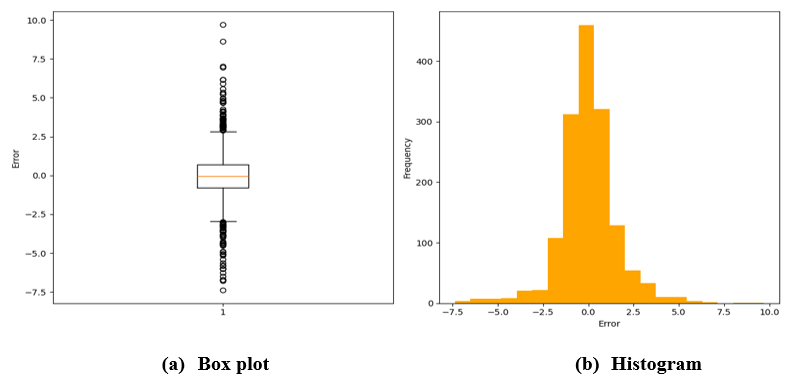
Figure 14 - Box Plot and Histogram for DT
Box plot illustrates the distribution of prediction errors to analyze the model’s residuals. Box plot is a standardized way of displaying the distribution of data based on five-number summary. Box plots are specifically useful for comparing the distributions across different groups, as it can generate clear visual summary and variability. In Figure 14 (a), the median error is very close to 0, meaning the model is unbiased on average. Besides, most the errors fall within a small range around 0, reflecting good overall accuracy. Hence, box plot of figure 13(a) performed well with most predictions having low error.
Figure 14 (b) shows the histogram of the DT. Histogram is a graphical representation of the frequency distribution of numerical data. It groups data into intervals and displays the frequency of data points within each bins using bars. The majority of errors fall within the range of -2 to +2, indicating satisfied accuracy for most predictions. The error distribution aligns well with the expectations of a model, with errors mostly concentrated near 0 and tapering off symmetrically.
b) Random Forest
Like DT, outcome for Random forest is demonstrated in the subsequent section. Figure 14 shows the regression performance for actual vs. predicted for RF.
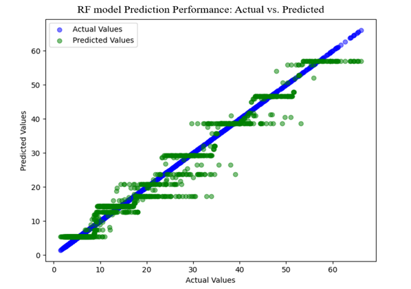
Figure 15 - Actual vs. predicted values for RF
The points in the figure 15, mostly cluster closely around the diagonal line, indicating that the model predictions closely match the actual values. This suggest that the regression model of RF has decent performance with minimal systematic bias. Moreover, the spread of points around the diagonal remains relatively consistent across range of values. This indicates uniform performance across the data range, with no significant outliers.
c) SVM
The Regression performance of SVM for actual vs. predicted is demonstrated in the figure 16. Here, the points align closely along with diagonal, indicating the models predictions are nearly identical to the actual values and there are no significant outliers or deviations in the model which hinder the performance of the model. Hence, the strong linear patterns confirms that the regression model has captured the relationship between he features and the target variable decently.
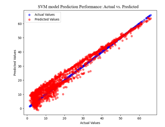
Figure 16 - Actual vs. predicted Values for SVM
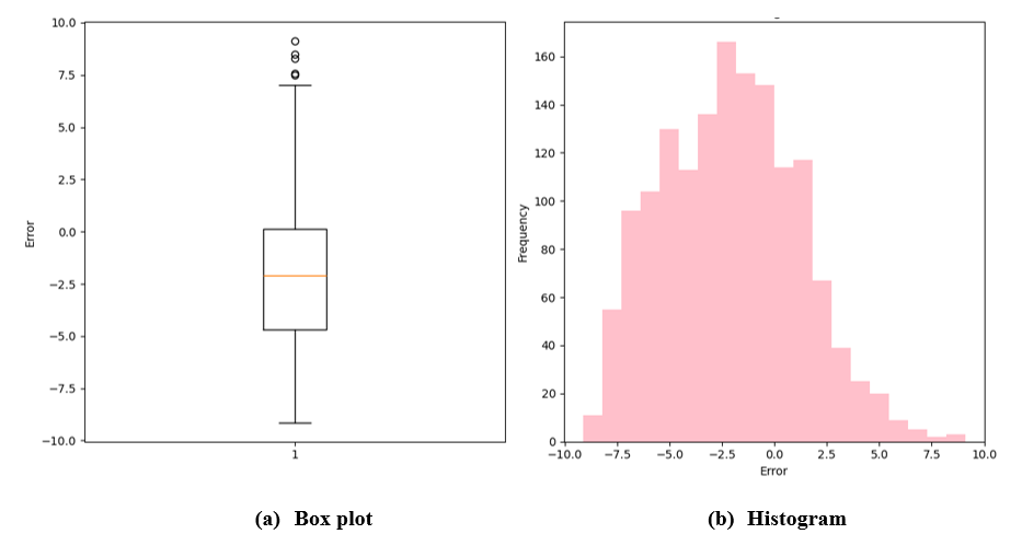
Figure 17 - Boxplot and histogram of SVM
Similarly, box plots and histogram for the SVM is illustrated in figure 17. Box plot visualizes the distribution of prediction errors, in which the medial (orange line) is very close to 0, indicating that the errors symmetrically distributed with no significant bias. Besides, the majority of the error values fall within a small range, roughly between -0.05 to +0.05, showing the model’s errors are generally small and few points below -0.1 are identified as outliers. These represent the cases where the model slightly underperformed. Likewise, Figure 16 (b) depicts the histogram of the model, in which the error distribution is symmetric and bell shaped centered on 0, which aligned with the expectations for regression model. Moreover, most errors are concentrated between -0.05 and +0.05, with very few extreme values. This indicated that the model’s predictions are consistently close to the actual values.
d) Proposed Model
Results obtained using proposed model is depicted in the subsequent section. Convergence curve obtained by the proposed model is illustrated in figure 18. Likewise, Figure 18 showcases the training loss, validation loss of the proposed model over 10 epochs. Convergence curve shows how the fitness cost evolve across generation during optimization process, x axis denotes the number of generations over time, where it spans from 0 to 2 generations, showcasing that the optimization converged very quickly. Likewise, y axis represents the fitness value during the optimization process. The flat line after generation 1 indicate the algorithm stability. Hence, the curve demonstrates that the optimization process is efficient and fast, requiring one generation to find the best solution
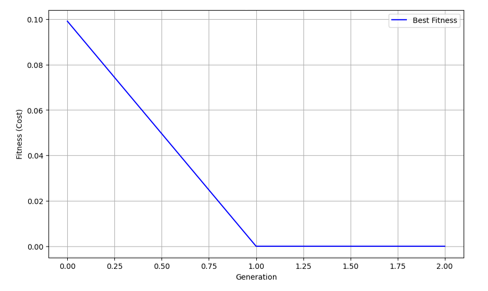
Figure 18 - Convergence Curve of the proposed Model
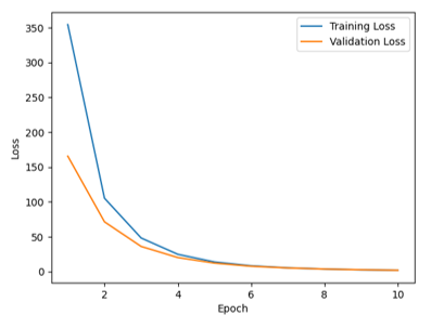
Figure 19 - Model loss of proposed Model
Figure 19 showcases the model loss plot, in which the blue curve represents the training loss and orange curve depicts the validation loss. Training loss starts by very high (around 350) and drops significantly in the forest few epochs. By epoch 5, the curve flattens and converges close to zero by epoch 10. This indicates that the model is learning efficient and minimizing its errors during training. For validation loss, the curve starts at a relatively lower value (about 150) and decreases steadily. By epoch 5, validation loss stabilizes and remains close to the training loss, depicting that the proposed model generalizes well to unseen data and is not overfitting. Therefore, the steady decrease of both curves and its convergence by the end of the training indicates well-trained model.
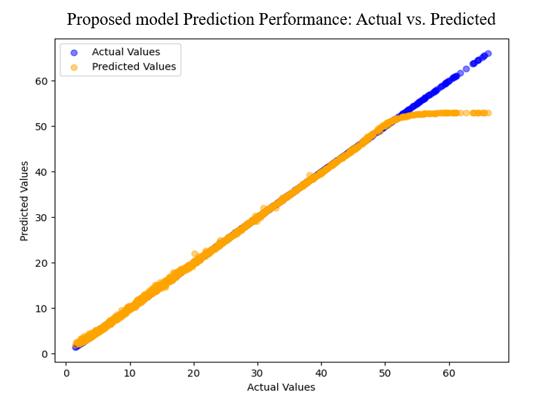
Figure 20 - Actual vs. Predicted Values of Proposed Model
Figure 20 showcases the actual vs. predicted values for the proposed model, in which the alignment of the points indicated a strong correlation between actual and predicted values, stamping its superior performance of the model. Moreover, the proposed model has captured the underlying patterns in the data accurately and precisely. Therefore, strong performance with minimal error spread and strong alignment between actual and predicted value have been unveiled by the model.
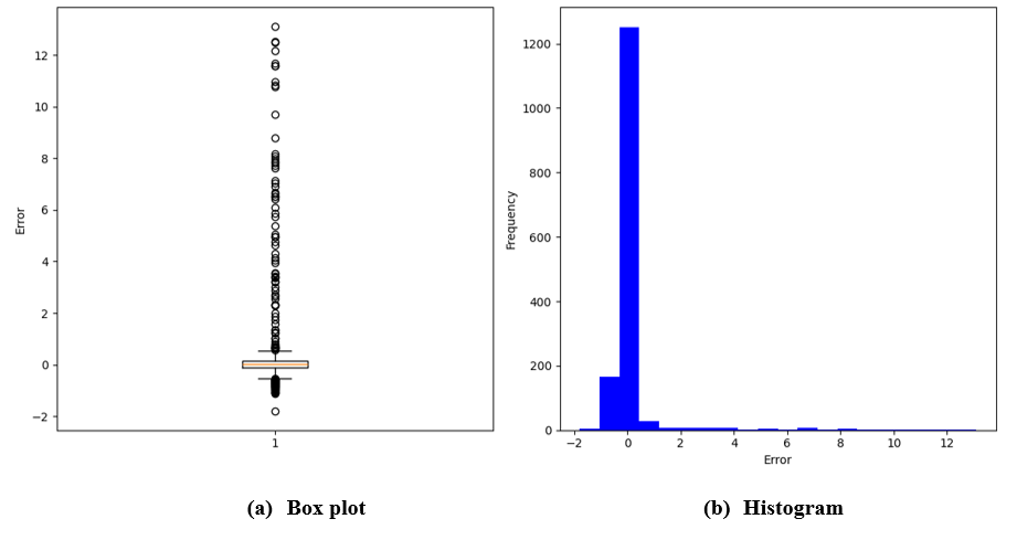
Figure 21 - Box plot and Histogram of Proposed model
Box plot of the proposed model is depicted in figure 21 (a). Where, errors are concentrated around 0, as evidenced by the narrow IOR (Interquartile Range). There are a few outliers, with errors extending up-to around +12 and slightly below -2. The low central tendency of errors exhibited that the majority of predictions are accurate and precise. Similarly, Figure 21(b) shows that histogram of the proposed model, in which a sharp peak near 0 reinforces that most predictions are highly accurate. Thus, the distribution is heavily skewed toward zero error, deliberated on the strong predictive performance.
4.2.1. Comparative Analysis
The performance of the proposed model is compared with existing ML models such as RF, SVR, and DT. This comparison is illustrated in a table 1 that highlights various performance metrics including MAE, MSE, RMSE and R².
| Metrics | RF | SVR | DT | Proposed Model |
|---|---|---|---|---|
| MAE | 2.1758 | 3.1816 | 1.0838 | 0.4179 |
| MSE | 8.7504 | 15.1145 | 2.5026 | 1.9380 |
| RMSE | 2.9581 | 3.8877 | 1.5819 | 1.3921 |
| R² | 0.9654 | 0.9403 | 0.9901 | 0.9923 |
SVR model has relatively high error metrics compared to other models. The MAE suggests that, on average predictions are off by about 3.18 units from actual values. The R² values of 0.94 indicates that approximately 94% of the variance in the dependent variable can be explained by this model. Likewise, DT model showed significantly lower error metrics than the SVR model, with an MAE of just 1.084, indicating more precise predictions on average. However, RF model performed better than SV model but not as well as the DT or proposed work. Its MAE is lower than that of SV bur higher than that of DT, indicating moderate accuracy in predictions with an R2 value.
Nevertheless, the proposed model stands out when compared to other models across all metrics with an exceptionally low MAE of just 0.418, indicating that its predictions are very close to actual values on average. The MSE and RMSE values are also notably low exhibiting minimal error in predictions and making it highly reliable for forecasting purposes. Moreover, R squared value of 0.992 indicates that proposed model exhibited an impressive 99.2% of the variance in the data.
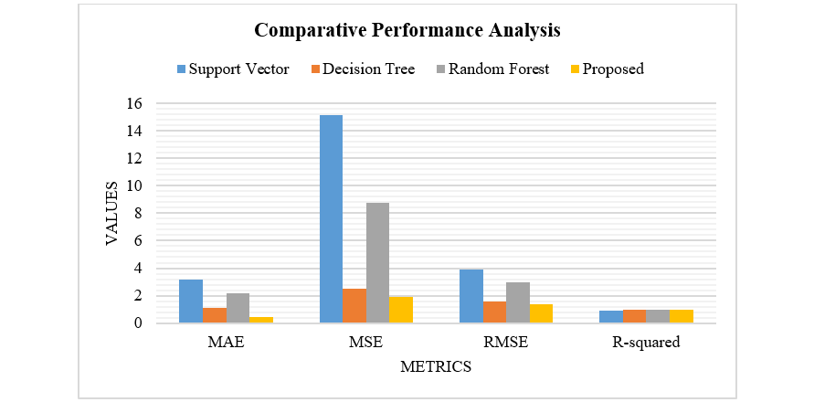
Figure 22 - Comparative Performance Analysis using Various Metrics
From the analytical outcome, it is very well defined that proposed model has delivered better performance than state-of-the-art models as proposed mechanism uses SWO with better exploration and exploitation phase, this enhanced exploration and exploitation phase enhances the process, by avoiding local optima and ensured a diverse set of candidate solutions. Hence, the overall outcome of the model shows the efficacy of the present research work in terms of decreasing the usage of power plant generators and its cost.
| Model | CO₂ Emissions (tons) | Reduction vs. Baseline (%) |
|---|---|---|
Baseline MG Operation (No Optimization) | 102.5 | – |
Decision Tree (DT) | 88.3 | 13.9% |
Random Forest (RF) | 84.6 | 17.5% |
Support Vector Regression (SVR) | 90.2 | 12.0% |
Proposed SWO + BiGRU | 68.7 | 32.9% |
Table 2 clearly demonstrates the superior environmental performance of the proposed SWO with BiGRU framework for microgrid operation. While traditional ML approaches like DT, RF, and SVR achieved better reduction in CO2 emissions compared to the baseline (13.9%, 17.5%, and 12.0% respectively), the proposed enhanced SWO with BiGRU model significantly surpasses them, achieving a remarkable 32.9% reduction in CO2 emissions. This translates to the lowest absolute CO2 emissions at 68.7 tons, indicating that the optimized BiGRU model is highly effective in minimizing the environmental impact of microgrid operations.
4.2.2. Scenario Analysis
In this context, the robust generalizability of the SWO–BiGRU framework was rigorously demonstrated through comprehensive scenario analysis encompassing diverse microgrid operating conditions. Specifically, the framework was evaluated across varying load demands (ranging from ±2.5% to ±10%), fluctuating seasonal renewable generation, and different diesel generator fuel cost profiles. Across all these scenarios, the model consistently exhibited high predictive accuracy (R² > 0.98) and maintained low error metrics, affirming its capacity to handle both typical and extreme operational circumstances without significant performance degradation. This extensive validation confirms that the SWO–BiGRU approach is not overfitted to specific operating regimes but can be effectively and reliably deployed in a wide array of real-world, dynamic microgrid energy management applications.
Discussion
In the present study enhanced SWO framework, incorporating PPCBO and FFSPM mechanisms, exhibits excellent scalability for microgrid optimization problems of increasing complexity, maintaining both rapid convergence and high accuracy. It outperforms state-of-the-art optimizers like GA [42], PSO [43], WOA [44], and IARO by achieving near-optimal solutions in fewer iterations and preserving solution diversity through targeted feature space reduction and adaptive diversity preservation, eliminating redundant fitness evaluations. This approach offers a favorable trade-off between computational cost and optimization quality, making it ideal for real-time microgrid energy management scenarios with limited optimization windows.
Additionally, the proposed research has achieved significantly lower RMSE values of 1.3921, outperforming the existing studies with RMSE values of 3.9 and 3.4 [45] [46]. Specifically, the existing study utilizing the HBO-LSTM technique reported an average performance with an RMSE of 3.9, whereas the proposed study demonstrated superior performance by employing the SWO algorithm, resulting in an RMSE of 1.3921. This notable improvement highlights the effectiveness of the SWO optimization algorithm in comparison to existing models that utilize HBO-LSTM [45] and ACO-NN algorithms [46]. Furthermore, the internal comparisons have illustrated that the proposed model outperforms traditional methods such as Random Forest, Support Vector Regression, and Decision Trees. This enhanced performance can be attributed to the integration of the SWO optimization algorithm during the feature optimization phase. Additionally, the proposed model employs an advanced DL architecture, specifically BiGRU, for the prediction process as BiGRU can process data in both forward and backward directions allows for a more comprehensive understanding of the input sequences compared to traditional algorithms that can only consider past states, thereby facilitating more effective strategies for carbon emission reduction. By doing so, proposed model overcomes the limitation of high error rates, vanishing gradient issue, computational complexity and overfitting of the model.
5. Conclusion
Proposed model effectively accomplished in reducing the CO2 emissions from power plant generator and focused on maximizing the use of renewable energy sources by ensuring that it is used optimally. Besides, it also emphasized on achieving optimal times to run the generator and decided when to charge the battery using renewable energy source, thereby reducing the cost. It was achieved by using the proposed SWO model, where algorithm dynamically adjusted the balance between exploration using PPCBO and exploitation using FFSPM based on the feedback from preceding iterations. This adaptability allowed it to respond to changing conditions in real-time, thereby being beneficial in environments where DG operate under varying loads and fuel qualities. Moreover, the incorporation of BiGRU model resulted in forecasting the energy consumption and practice of power in MG efficiently and optimized the cost and emission reduction, alongside BiGRU for accurate energy prediction, outperforming the traditional models. From the proposed work, the numerical outcome gained by the model are MAE of 0.4179, MSE of 1.9380, RMSE of 1.39212 and R² of 0.9923. Moreover, the framework significantly outperforms the traditional ML models like RF, DT and SVR in reducing CO2 emissions, achieving a remarkable 32.9% reduction compared to these existing approaches. This superior efficiency demonstrates the framework's effectiveness in minimizing the environmental footprint of microgrid operations. The future work should focus on further improving and refining the models by incorporating additional factors such as long-term monitoring and case studies. Besides, different optimization approaches will be reconnoitred to enhance the performance. Moreover, exploring the integration of social, economic, and policy aspects in low-carbon intelligent energy systems is crucial for sustainable development.
References
- A. Varshnry, J. S. Lather, and A. K. J. E. S. Dahiya, "Supply energy management methods for a direct current microgrid: A comprehensive review," vol. 6, no. 1, p. e578, 2024.
- A. Eskandari, M. Emamian, A. Nedaei, and M. Aghaei, "Digital twin technology in microgrid systems," in Digital Twin Technology for the Energy Sector: Elsevier, 2025, pp. 111-141.
- A. Akter et al., "A review on microgrid optimization with meta-heuristic techniques: Scopes, trends and recommendation," vol. 51, p. 101298, 2024.
- Y. Wang, Z. Wang, and H. J. J. o. C. P. Sheng, "Optimizing wind turbine integration in microgrids through enhanced multi-control of energy storage and micro-resources for enhanced stability," vol. 444, p. 140965, 2024
- A. Roy, S. Pramanik, K. Mitra, and M. J. W. J. o. E. Chakraborty, "Advanced hybrid neural network techniques for minimizing gas turbine emissions," 2024.
- A. Roy and M. Chakraborty, “Effects of Ship Emissions on Asian Haze Pollution, Health, and IMO Strategies,” Societal impacts, pp. 100055–100055, Mar. 2024, doi
- S. Dawn et al., "Integration of Renewable Energy in Microgrids and Smart Grids in Deregulated Power Systems: A Comparative Exploration," vol. 5, no. 10, p. 2400088, 2024
- W. Abdulrazzaq Oraibi, B. Mohammadi-Ivatloo, S. H. Hosseini, and M. J. A. S. Abapour, "Multi microgrid framework for resilience enhancement considering mobile energy storage systems and parking lots," vol. 13, no. 3, p. 1285, 2023
- A. Joshi, S. Capezza, A. Alhaji, and M.-Y. J. I. C. J. o. A. S. Chow, "Survey on AI and machine learning techniques for microgrid energy management systems," vol. 10, no. 7, pp. 1513-1529, 2023
- L. O. P. Vásquez, J. L. Redondo, J. D. Á. Hervás, V. M. Ramírez, and J. L. J. A. E. Torres, "Balancing CO2 emissions and economic cost in a microgrid through an energy management system using MPC and multi-objective optimization," vol. 347, p. 120998, 2023
- Y. W. Koholé, C. A. W. Ngouleu, F. C. V. Fohagui, and G. J. R. E. Tchuen, "Optimization of an off-grid hybrid photovoltaic/wind/diesel/fuel cell system for residential applications power generation employing evolutionary algorithms," vol. 224, p. 120131, 2024
- M. K. Patel, S. K. Verma, P. J. R. J. o. E. T. Sharma, and M. Sciences, "Advancements through AI Integration in Hybrid Renewable Energy Systems: A Review," vol. 7, no. 01, 2024
- M. Tahmasebi et al., "Optimal operation of stand-alone microgrid considering emission issues and demand response program using whale optimization algorithm," vol. 13, no. 14, p. 7710, 2021
- M. A. Majeed, S. Phichaisawat, F. Asghar, and U. J. I. a. Hussan, "Optimal energy management system for grid-tied microgrid: An improved adaptive genetic algorithm," vol. 11, pp. 117351-117361, 2023
- B. Dey, B. Bhattacharyya, and F. P. G. J. J. o. C. P. Márquez, "A hybrid optimization-based approach to solve environment constrained economic dispatch problem on microgrid system," vol. 307, p. 127196, 2021
- S. Hasan, M. Zeyad, S. M. Ahmed, M. S. T. J. E. P. Anubhove, and S. Energy, "Optimization and planning of renewable energy sources based microgrid for a residential complex," vol. 42, no. 5, p. e14124, 2023
- B. N. Alhasnawi et al., "A new methodology for reducing carbon emissions using multi-renewable energy systems and artificial intelligence," vol. 114, p. 105721, 2024
- M. Abdel-Basset, R. Mohamed, M. Jameel, and M. Abouhawwash, "Spider wasp optimizer: A novel meta-heuristic optimization algorithm," Artificial Intelligence Review, vol. 56, no. 10, pp. 11675-11738, 2023
- J. Sui, Z. Tian, and Z. Wang, "Multiple strategies improved spider wasp optimization for engineering optimization problem solving," Scientific Reports, vol. 14, no. 1, p. 29048, 2024/11/23 2024, doi: 10.1038/s41598-024-78589-8
- H. Das et al., "Enhancing software fault prediction through feature selection with spider wasp optimization algorithm," IEEE Access, vol. 12, pp. 105309-105325, 2024.
- S. Rajamand, M. Shafie-khah, and J. P. J. E. P. S. R. Catalão, "Energy storage systems implementation and photovoltaic output prediction for cost minimization of a Microgrid," vol. 202, p. 107596, 2022
- D. R. Nair, M. G. Nair, and T. J. E. Thakur, "A smart microgrid system with artificial intelligence for power-sharing and power quality improvement," vol. 15, no. 15, p. 5409, 2022.
- C. Ghenai and M. J. E. Bettayeb, "Modelling and performance analysis of a stand-alone hybrid solar PV/Fuel Cell/Diesel Generator power system for university building," vol. 171, pp. 180-189, 2019.
- M. S. Bakay and Ü. J. J. o. C. P. Ağbulut, "Electricity production based forecasting of greenhouse gas emissions in Turkey with deep learning, support vector machine and artificial neural network algorithms," vol. 285, p. 125324, 2021.
- H. Liu, Y. Wu, D. Tan, Y. Chen, and H. Wang, "CGAOA-AttBiGRU: A Novel Deep Learning Framework for Forecasting CO2 Emissions," Mathematics, vol. 12, no. 18, p. 2956, 2024
- A. A. Alhussan, M. Metwally, and S. Towfek, "Predicting CO2 Emissions with Advanced Deep Learning Models and a Hybrid Greylag Goose Optimization Algorithm," Mathematics, vol. 13, no. 9, p. 1481, 2025
- Z. Zuo, Y. Niu, J. Li, H. Fu, and M. J. A. S. Zhou, "Machine learning for advanced emission monitoring and reduction strategies in fossil fuel power plants," vol. 14, no. 18, p. 8442, 2024
- N. J. F. Pachauri, "An emission predictive system for CO and NOx from gas turbine based on ensemble machine learning approach," vol. 366, p. 131421, 2024
- M. Roslan, M. Hannan, P. J. Ker, R. Begum, T. I. Mahlia, and Z. J. A. E. Dong, "Scheduling controller for microgrids energy management system using optimization algorithm in achieving cost saving and emission reduction," vol. 292, p. 116883, 2021
- S. Shahpouri, D. Gordon, M. Shahbakhti, and C. R. J. I. J. o. E. R. Koch, "Transient NOx emission modeling of a hydrogen-diesel engine using hybrid machine learning methods," vol. 25, no. 12, pp. 2249-2266, 2024
- F. Ahmed, R. Al-Abri, H. Yousef, and A. M. J. I. A. Massoud, "An Optimal Energy Dispatch Management System for Hybrid Power Plants: PV-Grid-Battery-Diesel Generator-Pumped Hydro Storage," 2024
- O. D. Montoya, L. F. Grisales-Noreña, W. Gil-González, G. Alcalá, and Q. J. S. Hernandez-Escobedo, "Optimal location and sizing of PV sources in DC networks for minimizing greenhouse emissions in diesel generators," vol. 12, no. 2, p. 322, 2020
- P. Premadasa, C. Silva, D. Chandima, and J. J. J. o. E. S. Karunadasa, "A multi-objective optimization model for sizing an off-grid hybrid energy microgrid with optimal dispatching of a diesel generator," vol. 68, p. 107621, 2023.
- S. R. Shakya et al., "Estimation of air pollutant emissions from captive diesel generators and its mitigation potential through microgrid and solar energy," vol. 8, pp. 3251-3262, 2022
- A. M. Samatar, S. Mekhilef, H. Mokhlis, M. Kermadi, O. J. C. T. Alshammari, and E. Policy, "Optimal design of a hybrid energy system considering techno-economic factors for off-grid electrification in remote areas," pp. 1-29, 2024
- N. C. Alluraiah and P. J. I. A. Vijayapriya, "Optimization, design and feasibility analysis of a grid-integrated hybrid AC/DC microgrid system for rural electrification," 2023
- N. Rangel, H. Li, and P. J. A. E. Aristidou, "An optimisation tool for minimising fuel consumption, costs and emissions from Diesel-PV-Battery hybrid microgrids," vol. 335, p. 120748, 2023
- Z. Belboul et al., "Multiobjective optimization of a hybrid PV/Wind/Battery/Diesel generator system integrated in microgrid: A case study in Djelfa, Algeria," vol. 15, no. 10, p. 3579, 2022
- K. Almutairi, M. Almutairi, K. Harb, and O. J. F. i. E. R. Marey, "Optimal sizing grid-connected hybrid PV/Generator/Battery systems following the prediction of CO2 emission and electricity consumption by machine learning methods (MLP and SVR): Aseer, Tabuk, and eastern region, Saudi Arabia," vol. 10, p. 879373, 2022
- L. Kanaan, L. S. Ismail, S. Gowid, N. Meskin, and A. M. J. I. A. Massoud, "Optimal energy dispatch engine for PV-DG-ESS hybrid power plants considering battery degradation and carbon emissions," vol. 11, pp. 58506-58515, 2023
- F. Harrou, A. Dairi, A. Dorbane, and Y. J. R. i. E. Sun, "Energy consumption prediction in water treatment plants using deep learning with data augmentation," vol. 20, p. 101428, 2023
- X. Zhu, G. Ruan, H. Geng, H. Liu, M. Bai, and C. Peng, "Multi-objective sizing optimization method of microgrid considering cost and carbon emissions," IEEE Transactions on Industry Applications, vol. 60, no. 4, pp. 5565-5576, 2024
- K. Paul et al., "Optimizing sustainable energy management in grid connected microgrids using quantum particle swarm optimization for cost and emission reduction," Scientific Reports, vol. 15, no. 1, p. 5843, 2025
- H. Jouma, M. Mansor, M. S. Abd Rahman, Y. Jia Ying, and H. Mokhlis, "Influence of the demand side management on the daily performance of microgrids in smart environments using grey wolf optimizer," Smart and Sustainable Built Environment, 2024
- A. A. Ewees, M. A. Al-qaness, L. Abualigah, M. J. E. C. Abd Elaziz, and Management, "HBO-LSTM: Optimized long short term memory with heap-based optimizer for wind power forecasting," vol. 268, p. 116022, 2022
- S. Netsanet, D. Zheng, W. Zhang, and G. J. E. R. Teshager, "Short-term PV power forecasting using variational mode decomposition integrated with Ant colony optimization and neural network," vol. 8, 2022.