Flexible planning of low-carbon power systems under deep uncertainty
S. PUSCHEL-LOVENGREEN, S. MHANNA, P. MANCARELLA - University of Melbourne, Australia

Summary
The uptake of large-scale and distributed renewable energy sources and the electrification of different sectors around the world are engendering massive changes and creating unprecedented operational and planning challenges to power systems. These changes are bringing about increasing uncertainty as to what new network users will connect to the system, and when and where. For example, the recent Integrated System Plan (ISP) developed by the Australian Energy Market Operator (AEMO) even considers scenarios with large-scale adoption of hydrogen technologies for clean fuel export that might lead to a complete transformation and upsizing of the energy system. Planners are thus required to perform the daunting task of striking a balance between ensuring security and reliability and minimising cost while facing considerable long-term uncertainty. On the above premises, this paper aims to address a major open research problem of high immediacy: the development of planning methodologies and metrics to deal with the challenges associated with system-wide, long-term uncertainty. This includes the consideration of adaptive and flexible investment strategies that can enable the decision maker to optimally respond to unfolding uncertainty and assess the option value of proactive or delayed investments. To achieve this, stochastic optimisation modelling is applied here aiming at defining new methodological approaches and computational tools for planning of different transmission assets under deep long-term uncertainty. In turn, the results from the stochastic planning approach are compared with those obtained from deterministic approaches adopted by industry worldwide, such as least-worst (weighted) regret (LWR/LWWR). Various studies, conducted on real instances of the Australian power system as described in the most recent ISP presented in 2022, reveal new roles of different transmission investment options to deal with planning uncertainty. In particular, the results show that, relative to deterministic approaches, stochastic planning not only yields lower expected total cost (current and future investment in new transmission plus the future operation costs of the system), but also results in lower total costs (and thus in more efficient risk hedging) for the worst performing scenarios. This research has been conducted under the umbrella of the Global Power System Transformation Consortium (G-PST) initiative.
Keywords
Low-carbon power system planning, flexibility, stochastic optimisation, robust decision-making, least-worst regret, integrated system plan1. Introduction
As global power systems experience a surge in the adoption of distributed energy resources (DER) and renewable energy sources (RES) and the electrification of various sectors, significant changes and unprecedented challenges in planning and operation arise. The Integrated System Plan (ISP) [1] envisions that scenarios involving widespread implementation of new technologies might lead to a total transformation and expansion of the energy system. Consequently, planners face the task of striking a balance between ensuring reliability and minimising costs amid deep long-term uncertainty.
Major open research problems of high immediacy are the development of risk-aware planning methodologies and metrics to deal with the challenges associated with large-scale, long-term uncertainty. Practical steps in this direction have already been undertaken by a few system operators, most noticeably the National Grid Electricity System Operator (ESO) in the UK [2] and AEMO for the National Electricity Market (NEM) in Australia [1], through the adoption of metrics such as least-worst weighted regret (LWWR) [3], [4]. An even more powerful approach would consider how adaptive and flexible decisions could enable the decision maker to optimally respond to unfolding uncertainty and reveal the option value of proactive or delayed investments.
Most if not all transmission expansion methodologies used around the world by system planners are based on deterministic planning models, where many scenarios are analysed from a deterministic perspective. In some cases, the most advanced methodologies then use an additional metric to select the optimal plan for the system based on the results for the deterministic studies. Decisions made using the information obtained across multiple deterministic scenarios are being used in the UK, Australia and at least one jurisdiction in the US, through the so-called least-worst regret (LWR) and, more recently, LWWR. An in-depth analysis of these two approaches was conducted in [3], [4].
This paper studies how and why the results from a flexible plan stemming from stochastic planning model would differ from, and are potentially superior to, more established approaches such as LWWR. This is achieved by conducting a quantitative comparison, through case studies based on AEMO’s ISP 2022, between deterministic-based LWR and LWWR metrics and the stochastic planning approach introduced, with the aim of understanding the pros and cons of each approach.
2. Stochastic planning model
The planning of the system's expansion presents a challenge that demands careful consideration of operational details to evaluate investment options while facing the complexities associated with expanding power systems under uncertain conditions. In the context of stochastic planning the uncertain parameters (e.g., load, renewable energy capacity, retirements, investment and operation costs) in the expansion model are depicted through a scenario tree. This tree captures the variables' uncertainty while maintaining the physical correlation across the system's relevant variables and parameters. We have shown [5] the relevance of representing the complex nature of uncertainty in high detail to determine the investment options that can provide the highest value across scenarios.
In the illustrative example of Figure 1, the tree's nodes represent specific years in epochs and are organised into three scenarios (Scenario 1: N1-N2-N4, Scenario 2: N1-N2-N5, Scenario 3: N1-N3-N6), with each node depicting operation and investment for that year. Nodes 2 and 3 differ in expected demand and renewable capacity in year 2 (Y2). The paths between nodes represent branching in future uncertainty, modelled with probabilities that sum to 1. For example, if paths between node 1 and nodes 2 and 3 are equally likely, each has a probability of 0.5, whereas the transition between node 3 and node 6 has a probability of 1, as only one future is expected from node 3 onwards.
System operation is modelled through a set of representative days, weeks, or months, which are assumed to be independent. For instance, in Figure 1 the operation of each node is represented through three typical periods, which are labelled PX,Y, where X is the node number and Y is the period number. To clarify this even further, this means that the operation in node 1 will be represented by three typical weeks (could be days or months) of operation with hourly resolution. These three weeks are selected (for instance, through a bespoke clustering methodology) from the 52 weeks in the year under analysis for that node and could for example correspond to one week with the highest demand, one week with the lowest demand, and the one with average conditions. Each of the representative periods can have a different weight throughout the year. Investment decisions for new assets are made at each node of the tree.
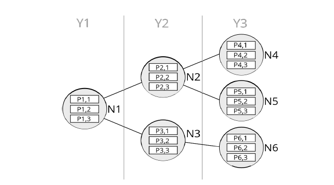
Figure 1 - Illustrative scenario tree
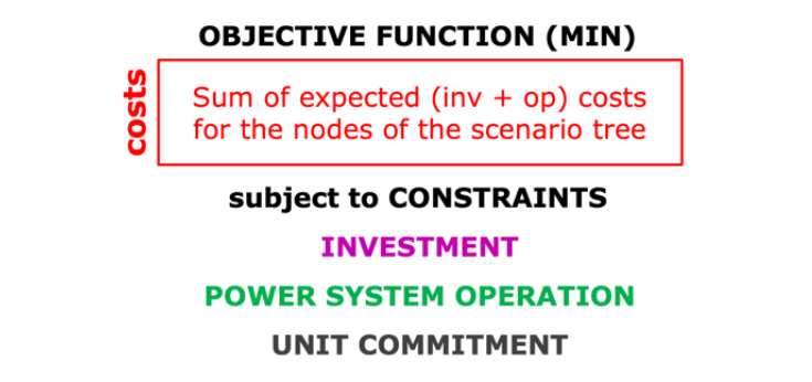
Figure 2 - Stochastic planning model
2.1. Expansion planning problem
This section describes the main components of the underlying mathematical problem that describes the expansion planning problem under uncertainty. First, Figure 2 depicts the general structure of the planning model. The optimisation problem aims to minimise the total expected costs associated with the investment and operation decisions made in each node of the scenario tree. The operation component of the total costs also includes the cost of not serving energy to the customers at any given period, which in the context of this study is valued at the current market price cap for the NEM.
This objective function is subject to a set of constraints that includes:
- Investment constraints: these include the so-called non-anticipativity constraints, which guarantee that an investment made at a certain node in the scenario tree will be present in the subsequent nodes connected to said node. These constraints also include the potential rules of investment across the portfolio of options, for instance, investment options that are mutually exclusive or investment options that must follow another investment option.
- Power system constraints: these correspond to all the constraints associated with power system operation, including energy balances, reserves, power flow, transmission limits, etc.
- Unit-commitment (UC) constraints: the operation of conventional units in the system is bound by their technical characteristics, for instance, ramping limits, minimum stable generation, start-up times, etc.
The structure of the problem presented in Figure 2 can be translated into a comprehensive mathematical problem, although here we do not introduce those details. For a detailed description of the investment and operation models used in this work, please refer to [6]. The objective function of the stochastic investment problems adds up all the investment and operation costs of the set of nodes (and associated representative weeks) in the scenario tree. Note that the operation of each representative week can be multiplied by a factor to reflect the weight of that week in the operation of the year associated with the node that contains it. These costs are discounted from the year associated with each node to a reference year using a given rate of return. Also, since the approach considers expected cost minimisation, each node is weighted by its probability of occurrence.
3. Deterministic-based approaches to transmission investment planning
Many system planners around the world use deterministic planning models for transmission expansion methodologies, in which they evaluate multiple scenarios from a deterministic perspective. In some cases, advanced methodologies include an additional metric to identify the best plan for the system,drawing from the results of these deterministic assessments. In the UK, Australia, and at least one US region, decisions are informed by data gathered from various deterministic scenarios, employing the LWR and, more recently, LWWR methods. LWR decisions operate based on the use of regrets as the indicator to the proximity to the best solution. The mechanics of LWR are described below:
- Select several scenarios and investment options to study.
- For each independent scenario determine the optimal portfolio of investment options that minimises the cost of that scenario.
- Using all the optimal portfolios (which we will call development paths) found in the previous set, determine the investment and operational cost resulting from applying each of those development paths to each of the scenarios under consideration.
- Using the matrix of costs, determine the specific development path from the set of development paths found before that produces the lowest (reference) cost for each scenario.
- Using such cost as reference, the regrets are calculated by determining the difference between the cost of each development path and the reference cost.
- For each development path, determine the worst (maximum) regret (that is, the maximum possible value in each column) that such development path can produce across all scenarios.
- The vector of worst regrets associated with each development path can then be minimised to determine which development path produces the “least-worst” regret in the set of paths under consideration (Figure 3).

Figure 3 - Path selection based on the minimum worst regret across development paths
A variant to the methodology presented before corresponds to multiplying the costs in Figure 3 by the probability of each scenario before determining the regrets. This approach yields the LWWR solution and aims to incorporate scenario probabilities in the LWR approach that otherwise manipulates results across scenarios assuming to be probability agnostic (which is equivalent to assuming the same probability of occurrence in all scenarios).
The approach to calculate LWR/LWWR presented in (i)-(vii) describes the general mechanisms of the procedure. However, there are various ways to define the candidate development paths. In (i)-(vii), the matrix of costs is built by determining the cost of applying the full development path found by optimising each scenario in a deterministic manner. This is something that system operators that use LWR/LWWR, like NGESO or AEMO, do differently.
4. Case study applications
The different studies on expansion planning presented in this paper use the information presented in the ISP 2022 [7]. The system under consideration corresponds to the Australian NEM as defined in the input assumptions database associated with the ISP [7].
The underlying data to describe the current and future system conditions is used directly from the ISP 2022 data. The studies conducted here only focus on making decision on transmission investment options, so the information on optimal generation capacity for the different technologies, retirement of synchronous units and storage capacity is obtained from the optimal development path found in the ISP 2022, which corresponds to the candidate development path 12 in that study. Figure 4a depicts the 10 subregions under consideration in the ISP for the expansion planning exercise. Figure 4b highlights the candidate lines (black segments) considered in the ISP 2022 (the picture excludes commercial solutions also considered in the ISP 2022).
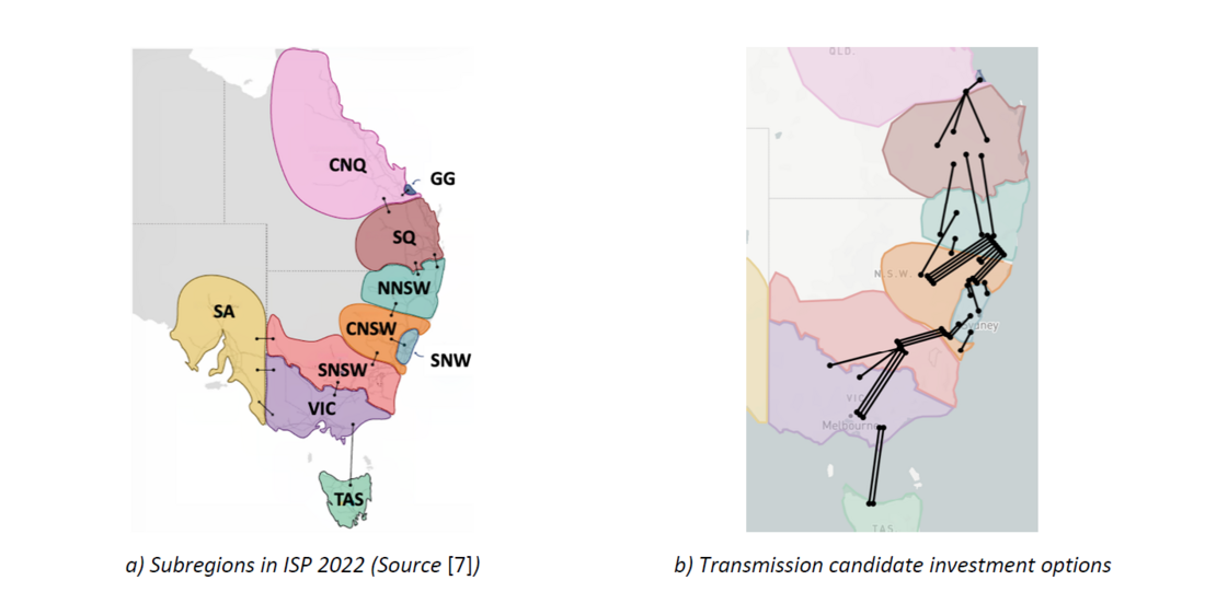
Figure 4 - NEM system regions and transmission candidate investment options modelled in the ISP 2022
The transmission system considers 11 existing links between the different subregions. The project EnergyConnect between SA and SNSW, although still under development, is considered to start operations in 2026. There are 34 transmission investment options (see Figure 4b) that consider different transfer capabilities across their boundaries and different investment costs.
The stochastic planning model has the capacity to model real transmission options, that is, the specific projects that are considered in the ISP and the relationships among projects. In this sense, the portfolio of options can be represented both considering mutually exclusive projects and must follow projects. The consideration behind mutually exclusive sets is that only one option can be built if this results in benefits for the overall expected cost minimisation objective of the problem. Must follow projects are represented as options that have to be in place in the system to build another option (simultaneous construction is also accepted). To focus on the transfer capacity requirements between boundaries, for simplicity the new links are not subject to Kirchhoff’s voltage law.
4.1. Scenario modelling
The case study applications conducted in this study consider a complex representation of future uncertainty built based on the four scenarios considered by AEMO in the ISP 2022. As discussed in [5], the more uncertainty is captured in the representation of the future, the more value can be identified for critical investment options. Figure 5 shows the structure of the multi-stage modelling approach adopted here, which was built using the information provided by AEMO for each of the scenarios under consideration in the ISP 2022, which include the Slow Scenario, Progressive Scenario, Step Scenario and Hydrogen (H2) Superpower Scenario. According to AEMO, these scenarios have a probability of occurrence of 4%, 29%, 50% and 17%, respectively.
Using the information provided for the 4 scenarios defined by AEMO, new, “intermediate” scenarios are created, in a way that the resulting scenario tree would more closely emulate potential “incremental” transitions across scenarios (for instance, to represent the possibility of transiting from the progressive to the step scenario between years 2027 and 2032, as shown in the scenario tree of Figure 5 for nodes 3 and 10). In the context of the studies presented here, the probabilities for these transitions are determined using a heuristic approach based on the original probabilities described for the 4 original scenarios. These probabilities can be modified to represent the view of the planner, and the values used here are illustrative.
The approach to apply the deterministic-based metric LWR follows the steps introduced in Section 3 is applied to the independent scenarios obtained by disaggregating the scenario tree. Each of those scenarios are considered independent deterministic scenarios and are used to find the candidate development paths needed to build cost and regret matrices. This process is illustrated in Figure 6.
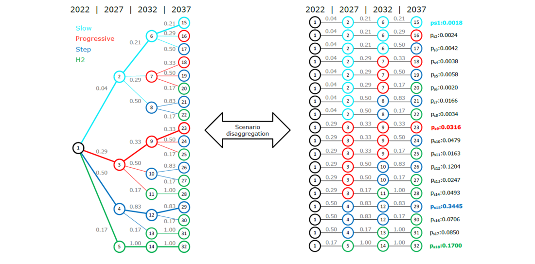
Figure 5 - 32-node scenario tree, corresponding to 18 “path” scenarios, used in the studies
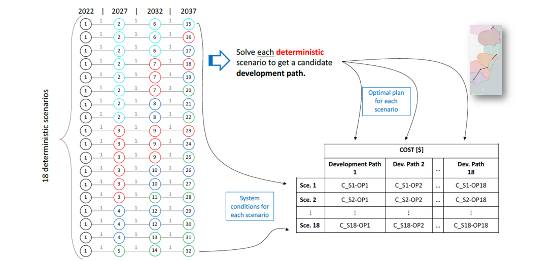
Figure 6 - Procedure to calculate the 18 deterministic development paths and build the cost and regret matrices
4.2. Operational data selection
Although off-the-shelf state-of-the-art MILP solvers can efficiently handle extremely large problems, the larger the problem, the slower the search process will be (and the larger the underlying computational infrastructure needs are). To help reduce the computation time, and in line with the methodological focus of this work, each year under analysis is represented by a subset of representative weeks selected among the 52 available weeks [1].
For each of the years selected to sample the scenarios, the following steps were taken to identify the subset of weeks closest to represent the operation of the 52 weeks: first, select the year and split all the corresponding data series into 52 weeks. Then, 6 weeks are selected (as a comparison, in Figure 1 the problem was structured using three representative weeks) to represent the periods with maximum and average demand, for different levels of renewable energy availability within the year at both system and state levels. The number of weeks could be increased or modified depending on the requirements of the study and the computational resources available [2].
4.3. Results
Using the stochastic model to tackle the definition of optimal investment in transmission lines for the NEM results in an optimal expected total (operation costs and investment in transmission assets) cost of $22.94 billion over the next 20 years. It is worth highlighting that it has been assumed that the lead time for each transmission investment option is 5 years, which means that the decision to invest made in a specific node of the tree depicted in Figure 5 results in the deployment of the new asset 5 years later. Figure 7 presents the distribution of costs for the scenarios contained in the scenario tree, where also a dashed line depicts the optimal expected cost (objective function of the problem).
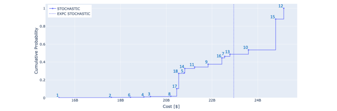
Figure 7 - Empirical cumulative distribution of scenario cost for the Stochastic case (numbers depict scenario id)
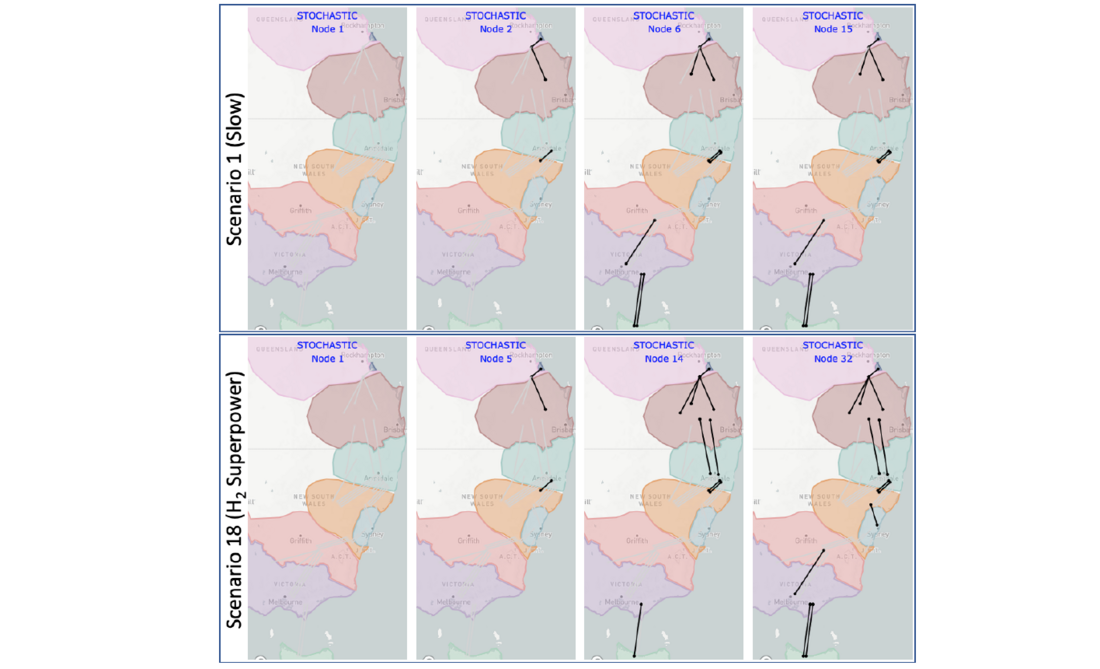
Figure 8 - Investment results in the Stochastic case for scenarios 1 (Slow) and 18 (H2 Superpower)
It can be seen that the total costs for the different scenarios cover a substantial range, starting at $15.3 billion for scenario 1 (corresponding to the Slow scenario in the ISP), going up to $25.13 billion for scenario 12 (from Figure 5, it corresponds to transiting to Progressive scenario in 2027 and then to the Step scenario onwards). Figure 8 shows the optimal stochastic investments observed in scenario 1 and scenario 18 (H2 Superpower). The investments that are progressed in 2022 become active in 2027, as seen in Figure 8, where both scenarios see the same active investments in 2027 (nodes 2 and 5 in the scenario tree), as they share node 1, where the decision to build is made.
Now we introduce the results for the deterministic-based approach. The cost and regret matrices resulting from applying steps (i)-(v) described in Section 3 are presented in Figure 9. The numbers have been rounded to the closest integer value for an easier interpretation of results. The diagonal of the cost matrix represents the total cost found in the process of determining the development paths for each scenario (optimal deterministic results for each scenario). For that reason, for any given scenario (row), the value in the diagonal of the matrix is the smallest possible. For instance, the value in the diagonal for scenario 10 is $21.3 billion, which results from finding the best investment options for the conditions in that scenario. On the other hand, the stochastic result for scenario 10 is $23.59 billion. This is because the stochastic solution factors in what is convenient for all the scenarios potentially unfolding in the form of the scenario tree, which leads to a compromise solution for all scenarios (thus possibly more costly than each specific corresponding deterministic counterpart).
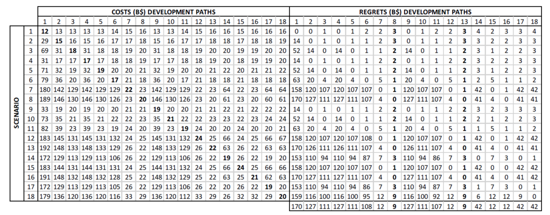
Figure 9 - LWR calculations (numbers have been rounded to the closest integer for ease of analysis)
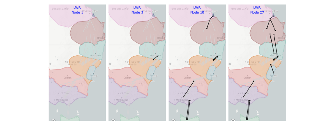
Figure 10 - Investment results for the optimal development path (scenarios 8/13) associated to the LWR metric
Following the steps (vi) and (vii) described in Section 3 it is then straightforward to identify the LWR solution for this study. In this case, the development path found for scenario 8 and scenario 13 are chosen by means of the LWR metric (although not presented here, when the analysis is extended to LWWR in this study case, the optimal results coincide). Both scenarios have the same deterministic development path (both scenarios are equal in all years except for year 2027 where scenario 8 is slow and scenario 13 is progressive), thus the worst regrets are the same, and occur in the case where the development path is deployed in the system, but scenario 18 (H2 superpower) unfolds.
It can be observed in Figure 10 that the optimal development path determined by LWR proceeds only transmission reinforcement in 2022 (CNSW-NNSW Option 6, as described in the ISP 2022) as opposed to the stochastic approach which proceeds three reinforcements (CNSW-NNSW Option 6, CNQ-GG Option 1, SQ-CNQ Option 2). In a first approach this may be seen as an advantage of the LWR approach, as it progresses less investment in the short-term. However, this is not necessarily correct from the perspective of the long-term results for the system and is a typical example of anticipatory investment that the stochastic planning model makes to create future investment optionality and hedge against risk due to uncertain futures.
Within the scope of this study, it can be asserted that a more accurate representation of the future aligns with the scenario tree depicted in Figure 5, rather than the disaggregated deterministic scenarios illustrated in Figure 6. Despite originating from the scenario tree, the deterministic scenarios are regarded as entirely independent representations of the future, as opposed to a cohesive perspective of the future embedded in the scenario tree. In this regard, the best approach to effectively evaluate the differences between the methodologies is to examine the performance of the optimal portfolio identified through the LWR metric (refer to Figure 10) by fixing the investment variables using the LWR solution values in the context of the stochastic problem addressed here for the scenario tree depicted in Figure 5. In fact, this result is already encompassed in Figure 9, specifically in the columns related to the costs of considering candidate development paths 8 and 13 across scenarios. Figure 11 expands upon Figure 7, incorporating the cumulative probability distribution of costs derived from the optimal development path (ODP) as determined by the LWR metric.

Figure 11 - Comparison between optimal stochastic results and the LWR optimal development path (ODP)
It is possible to see that the investment strategy resulting from the LWR approach yields results in which not only the expected total costs of transmission investment and operation are $1.5 billion more expensive, but also the worst performing scenario for the LWR portfolio is $4 billion more expensive than the worst performing scenario using the stochastic approach. On the other hand, stochastic planning exhibits the key feature of enabling (in case anticipatory) investments that can not only decrease the expected total cost, but also reduce the risk of excessively undesirable outcomes.
5. Conclusions
The comparative analysis of transmission investment decision-making approaches presented in this study demonstrates that the utilisation of distinct metrics and procedures for determining the optimal investment portfolio can lead to significantly divergent investment strategies under conditions of deep uncertainty.
The stochastic planning approach surpasses deterministic-based methodologies such as LWR/LWWR in addressing planning uncertainty, as evidenced by the case study of transmission planning for the Australian power system. The deterministic approach incurs higher expected total costs and considerably elevated costs for the worst-performing scenarios.
These outcomes arise from the distinct objectives of each metric: stochastic planning endeavours to minimise expected costs, resulting in an investment strategy with the lowest possible expected costs, specifically lower than those achieved by LWR/LWWR approaches, which prioritise minimising the worst regret. Notably, minimising the worst regret through deterministic analysis yields riskier portfolios, when looking at higher worst-case cost, compared to stochastic expected cost minimisation, suggesting that categorising LWR as a risk-averse metric may only be appropriate when regrets are the specific risk metric, while cost minimising stochastic planning generally brings less risky portfolios too when using worst-case cost as the risk metric. In fact, regrets represent a relative measure of scenario performance; consequently, they do not ensure the containment of impacts of extreme scenarios, as stochastic planning implicitly does, but merely reduce the worst difference between scenario costs.
Acknowledgement
This research has been conducted under the umbrella of the Global Power System Transformation Consortium (G-PST) initiative. The authors gratefully acknowledge the funding and support from the Commonwealth Scientific and Industrial Research Organisation (CSIRO) and the continuous feedback from AEMO and CSIRO.
References
- AEMO, “Integrated System Plan Methodology,” 2021. Accessed: Aug. 10, 2022. [Online].
- NGESO, “Network Options Assessment Methodology Electricity System Operator 2022-2023,”2022. Accessed: Sep. 30, 2022. [Online].
- P. Mancarella, S. Püschel-Løvengreen, C. Bas-Domenech, and L. Zhang, “Study of advanced modelling for network planning under uncertainty || Part 1: Review of frameworks and industrial practices for decision-making in transmission network planning,” 2020.
- P. Mancarella, L. Zhang, and S. Püschel-Løvengreen, “Study of advanced modelling for network planning under uncertainty Part 2: Review of power transfer capability assessment and investment flexibility in transmission network planning Report prepared for National Grid Electricity System Operator,” 2020.
- B. Moya, R. Moreno, S. Püschel-Løvengreen, A. M. Costa, and P. Mancarella, “Uncertainty representation in investment planning of low-carbon power systems,” Electric Power Systems Research, vol. 212, p. 108470, Nov. 2022, doi: 10.1016/j.epsr.2022.108470.
- S. Püschel-Løvengreen, “Security-constrained expansion planning of low carbon power systems,” 2021. Accessed: Aug. 03, 2022. [Online].
- AEMO, “2022 Integrated System Plan For the National Electricity Market,” 2022. Accessed: Sep. 29, 2022. [Online].
- I. J. Scott, P. M. S. Carvalho, A. Botterud, and C. A. Silva, “Clustering representative days for power systems generation expansion planning: Capturing the effects of variable renewables and energy storage,” Appl Energy, vol. 253, 2019, doi: 10.1016/j.apenergy.2019.113603.
- [1] In general, the selection of the input data is important to ensure adequate representation of system operation [8], which can have a substantial impact on the investment decisions derived from the long-term operation model.
- [2] The problem contains 29.64 million constraints and over 21 million variables (2176 binary variables). To close the mixedinteger linear gap below 1% Gurobi 9.0.3 took 21.5 hours. The problem was solved using 30 CPUs and 250GB of RAM