Regulating Service provision for intermittent inverter-based sources in tropical environments
Authors
J. SAUNDERS, P. TONKING - Power and Water Corporation
D. MARSHMAN - Market Reform

Summary
A consequence of the shift towards a low-carbon economy is that power systems are integrating a greater diversity of energy resources; electricity market design and associated power system management tools should therefore accommodate technologies with various technical and economic characteristics. For example, forecasting available capacity of variable renewable resources (wind and solar PV) is commonly recognised as being less accurate than thermal and storage technologies, and may require “firming” services when in generation mixes above moderate levels. This work explores a market design and methodology to determine requirements for a firming service for solar resources in particular, where such resources are unable to meet certain minimum forecast accuracy standards.
Under the approach, participants nominate a forecast root mean square error (RMSE) and commit to meeting that level of accuracy (avoiding a one-size-fits-all accuracy requirement). The system operator monitors and assesses the forecast errors across all solar participants and uses correlation coefficients between participant forecasts to determine an aggregate firming requirement, with the costs thereof allocated on the basis of contribution to overall requirements.
Others sources of variability - including demand and behind-the-meter (BTM) solar variations - are also accommodated. The distribution of demand variability is accounted for through expected changes in system demand over 30-minutes (which vary by time-of-day and year) and demand forecast errors around this expected value. This distribution then contributes to the total requirement.
This approach to determining a combined quantity of firming capacity for both utility-scale solar and demand (including BTM solar) is practicably implementable, having been developed with regard to a real-world power system, for which a case study of firming requirements is presented (including implementation considerations and refinements).
Keywords
Capacity Forecasting, Regulating Frequency Control Ancillary Service (R-FCAS), Contingency Frequency Ancillary Service (C-FCAS), Firming, utility-scale renewable generators , Root Mean Square Error (RMSE)1. Introduction
Globally, power systems are increasingly subject to substantial growth of intermittent generating capacity such as utility-scale solar and wind resources, whilst conventional fossil fuel generators are reaching end-of-life. Due to dependence on short-term weather conditions – mainly solar irradiance – the variability and uncertainty in solar generation can pose challenges for power system integration, especially where intermittent generators represent an increasing proportion of the power system capacity [1].
These challenges are particularly acute in smaller capacity non-interconnected power systems with peak demand of below 500 MW and a correspondingly low number of generating units. Hence, the variability of any one unit may have a disproportionately large impact on system frequency, compared to a larger system that can better absorb variability by virtue of having more diversified reserve and inertia resources. Further, under low load conditions, a limited number of thermal units may be online, limiting the availability of these services that can be used to mitigate imbalances in generation and system load.
Another consideration for renewable integration in power systems located in tropical and equatorial regions is that it is largely dependent upon solar PV, whereas other systems have broader renewable options such as wind and hydro resources. These non-interconnected power systems are characterised by generation being likely located within a small geographic area, meaning the same weather patterns will affect all solar plant, resulting in higher overall variability in supply availability. Given these attributes and considerations, integrating high volumes of renewable energy in these power systems requires careful consideration of impacts on system security.
2. The Need for a Firming Service
For non-interconnected regulated power systems there is a need for capacity forecasting requirements and accuracy standards to apply to generating units so that power system security could be maintained at all time [2]. Technical codes (such as within the Northern Territory of Australia) requires generators to submit forecasts at five-minute granularity over a 24-hour horizon. These requirements help to ensure the power system can be operated securely by providing a framework for making unit commitment decisions in the 30 minute time horizon it takes to start the next generating unit [3]. With the entry of weather-dependent utility-scale solar generation, concerns regarding the ability of these generators to meet the applicable forecasting accuracy standards have been raised. Hence it may be necessary for additional capacity to be available to firm solar forecast errors, with this referred to as a firming service. Note that over-forecast errors are the primary concern for system security, while under-forecasts would represent a loss in economic efficiency.
Firming could be provided individually by each solar farm, or specified as an essential system service, and obtained centrally from third-party providers by the system operator. This latter option would allow for combination of the firming service with the need to regulate operational demand variability, using a combined regulating frequency control ancillary service (R-FCAS). For this approach, the quantum of the required R-FCAS would be determined considering the individual drivers of power system variability, being solar forecast errors and demand variability (with the latter including distributed solar generation – i.e. rooftop PV). This would allow a given volume of R-FCAS to be procured. Recovery of the total R-FCAS costs would occur separately, with a proportion allocated to the firmed solar generators (in proportion to their forecasting errors), and the remainder allocated to loads. While this approach may carry some operational efficiencies (namely the combined service for firming and demand regulation), it requires an approach to determine the firming and R-FCAS requirements, as well as other implementation considerations discussed below.
3. Approach to Determining the Firming Requirement
A probabilistic approach is proposed to determine the quantum of required R-FCAS to meet the firming and regulating requirements because of the uncertain nature of forecast errors. Under this approach, participants that cannot meet the codified forecasting standard would nominate the accuracy to which they are able to forecast. The power system operator would then use participant’s nominated accuracy to determine the R-FCAS requirements, in the following process (see Figure 1):
- Error distributions for each error source are assumed to be normally distributed [1], and are specified based on:
- Solar participants that require firming nominating the root-mean square error of their forecasts.
- The system operator determining the root-mean square error of operational demand forecasts.
- The system operator determines correlation coefficients between each error source, with this expected to be largely dependent upon the distance between solar sites.
- The system operator then constructs a system-wide forecast error distribution, using the information from the previous steps.
- The R-FCAS requirement to meet a percentile (e.g. 99%) of the system-wide forecast error distribution.
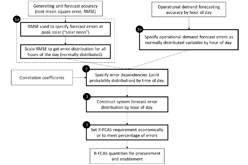
Figure 1 - Methodology overview
Under this approach, the requirement is determined by the (in)accuracy of participant’s nominated forecast ability. If a participant nominates a relatively low forecast accuracy, overall requirements would be relatively high, but that participant’s cost allocation would also be higher. Therefore, participants are incentivised to improve forecast accuracy, where practically possible.
Inclusion of correlation coefficients means that requirements would be expected to be higher if solar farms are not geographically dispersed.
The methodology is computationally simple and includes a direct link between the R-FCAS requirement and the individual sources of forecast uncertainty. Because of this simplicity, it would not be burdensome to repeat the exercise for different seasons (wet or dry seasons) or types of weather (clear and sunny, overcast, or partly cloudy), where these are expected to affect forecasting capability. This methodology is intended to inform procurement decisions – in an operating timeframe, additional tools may be needed to inform the volume of R-FCAS that is appropriate given factors such as weather forecasts, forecast demand variability as well as any immediate issues encountered by the system operator.
Participants would then submit their forecast availability as required in the technical codes, and the accuracy of the firmed participant’s actual forecasts would be assessed against their nominated accuracy over a defined period (e.g., quarterly or annually). If a participant’s forecasts are less accurate than was originally nominated, it may be subject to being de-rated/curtailed (if needed for system security) and/or allocated a greater proportion of the R-FCAS costs, particularly if procurement of additional firming capacity is then required.
4. Assessment of Required R-FCAS Volume and Considerations for Implementation
To gain an understanding of the approximate quantum of R-FCAS that would be required with implementation of centralised firming, analysis of utility-scale solar forecast errors and demand variability for a small power system was undertaken. This analysis considered firming for a number of solar farms which are currently being commissioned, with a combined capacity of 55 MW, and also considered correlations between forecast errors for each solar farm. Correlations were initially estimated using historically estimated and published values undertaken in a body of global research undertaken by the Lawrence Berkley National Laboratory [4].
Variability in 30-minute changes in operational demand was found to have a bi-modal nature, with a much broader (or uncertain) range of possible outcomes occurring during daytime periods (see Figure 22). Operational demand variability was also greater during the wet season, particularly for afternoon hours – this is thought to reflect afternoon storms that occur during the wet season.
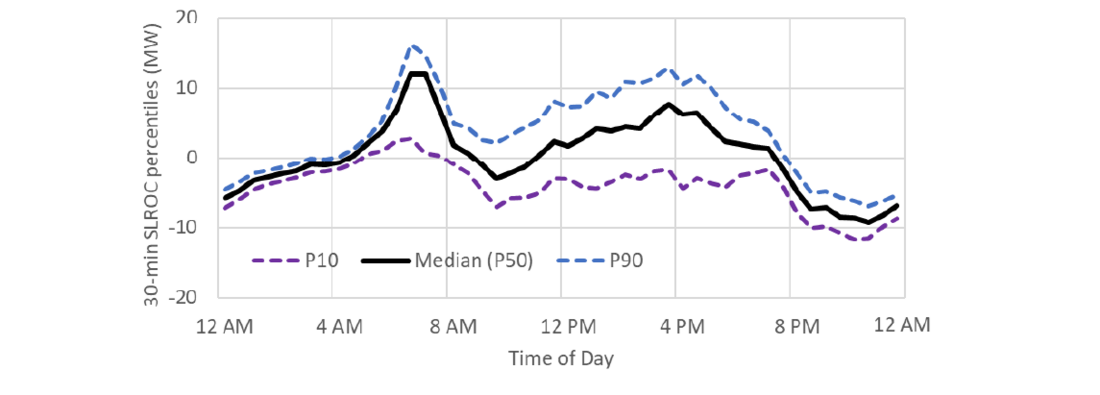
Figure 2 - Percentiles of 30-min System Load/Demand Rate of Change (SLROC) (wet season, 2021/22)
The magnitude of the solar forecast errors was found to be relatively constant across the majority of the daytime (excepting sunrise and sunset, where errors are lower than for other day-time periods). However, as for demand variability, the magnitude of the solar forecast errors was largest during the wet season. When solar forecast error distributions are combined with the distribution of demand variability, required R-FCAS capacity can then be determined. Resulting R-FCAS requirements for the dry and wet seasons in 2021/22 are shown in Figure 3, where:
- The grey line indicates the expected movement in operational demand – i.e., it captures the typical daily patterns such as morning and afternoon ramp ups (7 AM and 4 PM), and the night-time ramp down (from 8 PM). Note that negative values indicate that demand is expected to be ramping down in such periods.
- The purple line indicates the uncertainty in the expected demand movement, and is highest during day time periods, as also shown in Figure 2.
- The blue line indicates utility-scale solar forecasting errors, which are only non-zero in daylight hours.
- Finally, the thick black line combines the three previous quantities (note that this is not a direct sum), and represents the estimated total R-FCAS requirement to firm utility-scale solar and manage demand variability at the 99th confidence level. A minimum requirement of 5 MW is applied, in line with the System Control Technical Code.
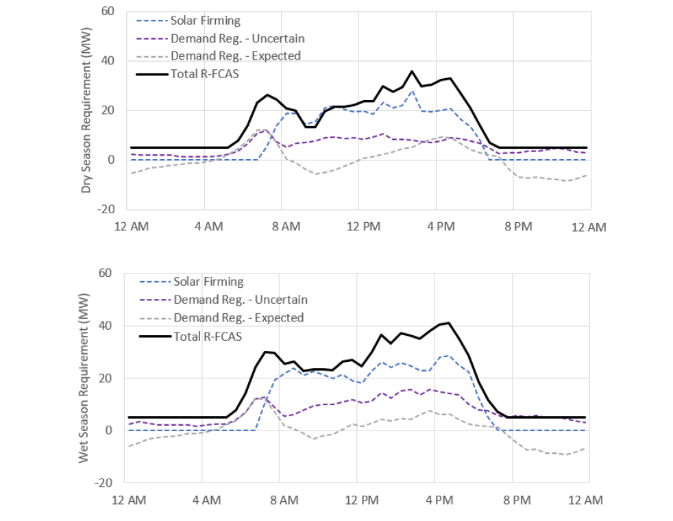
Figure 3 - Solar firming, demand regulation and total R-FCAS requirements, 2021/22 wet and dry seasons
For 2021/22 with 55 MW utility-scale solar generation, the wet season, daytime R-FCAS requirements are found to be within the range of 40 – 45 MW, while slightly reduced requirements of 35 – 40 MW apply for the dry season. The greatest requirements apply from mid to late afternoon, when demand is ramping up, and there is substantial uncertainty in available solar generation.
For comparison, in operating the power system, without the incorporation of solar farms, the traditional dynamic requirement on available R-FCAS, being the greater of 5 MW and the anticipated System Load Rate of Change (SLROC) over 30-minutes, with this latter value reaching up to currently approximately 17 MW or more. Therefore, centralised firming requires significant increases in regulation capacity relative to that required to manage demand-side fluctuations alone.
However, the centralised firming approach (a firming service is used to absorb forecast errors netted over the system) reduces requirements compared to a decentralised approach where participants locally balance forecast errors without any netting. This is because when one farm is over-forecast, another farm (or demand) may be under-forecast, reducing net error. Considering the four solar farms in this case study, centralised firming allows for a ~30% reduction on firming requirements under the decentralised approach. This diversity benefit would be expected to grow with both the number of solar farms, and increases in their relative geographic dispersion.
It is emphasised that this study considered 55 MW of utility-scale solar capacity – as solar capacity grows, the required quantum of R-FCAS would also be expected to increase. Indeed, it was found that growth in behind-the-meter solar in the system studied resulted in increased R-FCAS requirements of up to 52 MW in 2030-31.
5. Shortages of R-FCAS – the C-FCAS boundary
As the approach to setting the R-FCAS quantity is probabilistic in nature, and has been selected based on the estimated 99th percentile [2], there may be occasional extreme forecast errors that result in shortages of R-FCAS. In the first instance, it would then be necessary to deploy additional reserves (e.g., contingency FCAS – C-FCAS) in such events. This section provides some insight into the magnitude of such events, and whether they could be accommodated by the power system. The rationale for choosing the 99th percentile is based on the risk tolerance of the System Operator. In determining an extreme forecasting error as a contingency event there must be equivalence to the occurrences of conventional generator contingency events. This study assessed the occurrences of generator unit trips over a 12 month period to benchmark the R-FCAS - C-FCAS boundary.
Figure shows the highest 1% of a) the solar farm forecast errors (black), b) the system load variations (blue), and c) the total deviation (grey), being the concurrent solar forecast error and system load variation in an interval. Note that the latter is not simply the sum of the former two quantities. For example, a very large solar forecast may not result in a significant total deviation if the system load change is small, or even negative at the same time. On the other hand, a moderate solar forecast error and moderate system load change that occur simultaneously could – in combination – cause an R-FCAs shortage.
First considering the solar farm forecast errors, the figure indicates that the 1% largest errors are relatively flat – this is a consequence of the forecast errors frequently being large relative to the farm capacity. The solar farm capacity is an upper bound on the solar farm forecast error, and hence the distribution is capped or 'truncated'.
In contrast, over the highest 1%, the system load changes are typically slightly smaller than the solar farm forecast errors, but the largest system load changes exceed the largest solar forecast errors. The largest change over 30-minutes is approximately 35 MW, but a single 5-minute change of approximately 40 MW was observed in the dataset. Note also that the figure also shows only the system load changes in the upwards direction (i.e., increasing underlying demand or decreasing BTM solar output). The largest system load changes in the downwards direction are comparable to those in the upwards direction.
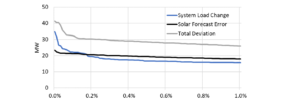
Figure 4 - Highest 1% of solar forecast errors, system load variations, and combined deviations
Finally, the grey line in Figure shows the top 1% of the combined, or total, deviations. A large deviation may result from an extreme solar forecast error or system load change, but may also occur where there is a moderately large and simultaneous contribution from both. In the latter case, neither may be problematic in isolation – it is the fact that they occur at the same time that causes a large deviation.
6. Practical Learnings and Refinements
6.1. Implications of constrained dispatch on firming requirements
The proposed approach determines firming requirements under the assumption that the output of generators is not constrained by grid constraints such as thermal transmission constraints, or simply because of economic curtailment. Determining the real time R-FCAS requirement under security-constrained economic dispatch needs to be investigated from an operational and market implementation perspective. The more constrained the generator the less firming is required, which may in turn reduce the number of thermal or storage resources that must be available.
A probabilistic optimisation could be used, allowing more complex generator costs and constraints to be incorporated. The objective function would be the cost of dispatching generators to meet load and to supply the firming service (and meet other ancillary service requirements). The R-FCAS needs would be represented probabilistically, based on a cumulative distribution function from Monte Carlo Analysis.
The level of firming service that is committed would be a variable to be optimised, given the distribution of possible solar forecast errors. This variable would be determined principally through the trade-off between the cost of reserving capacity for the firming service, and the cost of not being able to supply power to make up for forecasting errors that exceed the procured amount of the service, but would consider other costs and decisions, e.g. start-up costs, storage charge and discharge, and so on.
This way the optimisation may choose to curtail solar where this is more economical than procuring additional firming service – for example under high-solar, low-load conditions. However, the additional complexity of such a technique to the overall dispatch and scheduling process requires further consideration as an associated body of research.
References
- S. R. Sinsel, R. L. Riemke and V. H. Hoffmann, “Challenges and solution technologies for the integration of variable renewable energy sources—a review,” Renewable Energy, vol. 145, pp. 2271-2285, 2020.
- B. Mohandes, M. Shawky El Moursi, N. Hatziargyriou and S. El Khatib, “A review of power system flexibility with high penetration of renewables,” IEEE Transactions on Power Systems, vol. 34, no. 4, pp. 3140-3155, 2019.
- P. Meibom, R. Barth, B. Hasche, H. Brand, C. Weber and M. O'Malley, “Stochastic optimization model to study the operational impacts of high wind penetrations in Ireland,” IEEE Transactions on Power Systems, vol. 26, no. 3, pp. 1367-1379, 2010.
- T. E. Hoff and R. Perez, “Modeling PV fleet output variability,” Solar Energy, vol. 86, no. 8, pp. 2177-2189, 2012.
- R. Doherty and M. O'Malley, “A New Approach to Quantify Reserve Demand in System with Significant Wind Capacity,” IEEE Transactions on Power Systems, vol. 20, no. 2, pp. 587-595, 2005.
- M. A. &. K. D. S. Ortega-Vazquez, “Estimating the spinning reserve requirements in systems with significant wind power generation penetration.,” IEEE Transactions on power systems, vol. 24, no. 1, pp. 114-124, 2008.
- M. Black and G. Strbac, “Value of bulk energy storage for managing wind power fluctuations,” IEEE Transactions on energy conversion, vol. 22, no. 1, pp. 197-205, 2007.
- [1] Demand and solar forecast errors are assumed normally distributed, as in other studies e.g., [5], [6]. This assumption of course will not perfectly hold with real forecast errors. To the extent that distributions have material non-normal components, this can be accommodated, such as by increasing the standard deviation to capture longer tails, as in Black et al. [7]
- [2] In practice, this value may depend on policy settings, the value of customer reliability, and availability and costs of responsive capacity