Impact of Grid-Forming Inverters on Frequency Control of a Grid with High Share of Inverter-Based Resources
Authors
A. JALALI, E. FARAHANI, M. DELAC, N. MODI - Australian Energy Market Operator (AEMO), Australia

Summary
Increasing penetration of inverter-based resources (IBRs) and decreasing number of online synchronous generators (SGs) increases the complexities of managing stable controls of voltage and frequency.
Grid-Forming (GFM) inverters are gaining growing attention, owing to their potential capability to mitigate many of the issues associated with high IBR penetration. Most GFM inverters’ control philosophy attempts to maintain an internal voltage reference which is constant in the sub-transient to transient time frames. This provides a degree of stability in the voltage and frequency. More specifically, the constant internal voltage reference enables GFM inverters to emulate the inertial response of SGs by providing instantaneous active power response opposing frequency changes in the grid. Inertial response can be seen in contrast with Fast Frequency Response (FFR) provided by grid-following (GFL) inverters which requires measurement, detection, processing, filtering, and activation that result in a finite, although small, delay.
Virtual machine mode (VMM) is a specific control strategy for GFM inverters in which the dynamics of conventional SGs are modelled in the inverter control system. VMM allows for setting parameters like inertia and damping constant in the GFM plant. In Australia, several grid-scale battery energy storage systems (BESSs) are either operational or in the process of connecting to the grid. It is expected that a portion of the future BESSs will use GFM control strategies, including VMM.
In this paper, contribution of a GFM BESS (using VMM control) and a GFL BESS to the overall frequency stability of the power system is investigated and compared for a large-scale power system. The impacts of the inertia constant, damping coefficient, and droop constant of the GFM inverter on the frequency stability of the grid are also investigated. It is shown that the system strength support provided by the GFM inverter can enhance the frequency stability of the grid by improving the fault ride-through behaviour of the nearby IBRs. Finally, the grid’s “effective inertia” is calculated and compared for cases with GFM and GFL inverters. Results indicate that GFM inverters can notably improve the frequency stability of the grid. They do this not only through their inertial response, but also by providing system strength to nearby IBRs and improving their fault ride through performance. Also, results show that the right combination of inertia and damping constants needs to be used in the GFM inverter control system to avoid degrading the system damping.
Keywords
Grid Forming Inverter, Virtual Machine Mode, Inertial Response, Fast Frequency Response, Effective Inertia, Frequency StabilityAEMO Australian Energy Market Operator
BESS Battery Energy Storage System
FFR Fast Frequency Response
FRT Fault Ride Through
GFL Grid Following
GFM Grid Forming
IBR Inverter-Based Resources
NEM National Electricity Market
PLL Phase-Locked Loop
RoCoF Rate of Change of Frequency
SC Synchronous Condenser
SG Synchronous Generator
VMM Virtual machine Mode
VSG Virtual Synchronous Generator
1. Introduction
Australia’s National Electricity Market (NEM) is at the global forefront of energy transition with an unprecedented increase in the penetration of renewable inverter-based resources (IBRs). The instantaneous penetration of IBR generation in the South Australian (SA) region of the NEM, for example, has exceeded 140% of the operational demand at some operational periods [1].
The fast-growing penetration of IBR in the NEM grid has led to an inevitable decline in the number of online synchronous generators (SGs), which for long have been the conventional means of voltage and frequency control in the NEM [1]. The declining number of SGs has led to a steady decrease in the system strength, required for stable operation of grid-following (GFL) IBRs, as well as the level of synchronous inertia, necessary to limit the rate of change of frequency (RoCoF), in the NEM.
Maintaining a minimum number of SGs online and installing synchronous condensers (SCs) are some solutions implemented by the Australian Energy Market Operator (AEMO) in some NEM regions, mainly to maintain the required level of system strength [2, 3]. This also assists in maintaining a minimum level of synchronous inertia in the grid. Despite this, system strength and frequency control related issues have increasingly been witnessed in the NEM power grid [4, 5].
Grid-Forming (GFM) inverters are the new generation of inverters which use advanced control methods to stably synchronise with the external grid. Unlike GFL inverters, GFM inverters function as a voltage (rather than current) source and do not rely on SGs for their stable operation [5], [3]. GFM inverters generate their own internal reference voltage waveform and hence do not require phaselocked loop (PLL)-based measurement of the grid’s phase angle and frequency. As a result, they are not susceptible to PLL-related instabilities which typically happen to GFL inverters under low system strength conditions [3, 6]. Although GFM inverters’ capabilities such as system strength, fault current support, system restart contribution, and standalone operation during islanded conditions are also of high interest to the NEM, the focus of this paper is mainly the impact of GFM inverters on the frequency stability of the grid.
Synchronous inertia is considered as the main means of opposing abrupt changes in the SGs’ rotor speed and hence frequency during the network disturbances, via the immediate and inherent release of the rotational kinetic energy stored in the rotating masses of SGs [7]. Inertial response is critical for limiting the RoCoF immediately after a generation-load imbalance. This buys time for other frequency control measures to respond to the frequency deviation.
In the absence of sufficient inertia, fast frequency response (FFR) can assist in limiting the RoCoF. FFR is an intentional, controlled, and rapid increase or decrease in active power in sub-second time scales to correct frequency deviations [8]. FFR provision, however, requires measurement, detection, processing, filtering, and activation and hence characterizes an inherent delay [3, 6, 9]. Even though FFR mitigates the need for limiting the size of the largest credible contingency at low-inertia grids, it cannot fully replace the physical inertia [3, 4].
GFM inverters emulate the inertial response of SGs (so-called synthetic inertia), mainly by keeping their internal reference voltage phasor constant in the sub-transient to transient timeframe [9-12]. Unlike FFR, which is proportional to the frequency deviation, the inertial response is mainly driven by RoCoF [11, 13]. Virtual Machine Mode (VMM) concept, first proposed in [14], is a control strategy for GFM inverters in which the dynamics of SGs (swing equation, damping and inertia constants, droopbased governor response, etc.) are included in the inverter’s control system [3]. Making the most of the VMM implementation requires power and energy headroom as well as extra current capacity [15].
It has been demonstrated by several practical applications on small islanded systems that with a certain share of GFM inverters (with energy buffer), the minimum required level of rotational inertia or reliance on SGs can be lowered [3, 4, 11]. The 30 MW ESCRI battery energy storage system (BESS) in SA [12, 16] and the 69 MW Dersalloch wind farm in Scotland [4], for example, have demonstrated GFM inverters capabilities in the operation of a MW-scale island (including a grid-scale wind farm) and extraction of synthetic inertia from wind turbine blades, respectively. Despite these, the GFM inverters’ capabilities have not yet been demonstrated for large power systems [4].
In Australia, several grid-scale BESS are either operational or in the process of connecting to the grid. AEMO sees this as a window of opportunity and recommends prioritising the deployment of GFM capabilities on the future BESSs [4].
In the literature, GFM inverters have recently been receiving growing attention. In [17], the frequency responses of some GFM control methods are compared, using a small IEEE 9-bus test system. It is shown in [17] that all GFM control methods, in general, provide a positive impact on frequency stability metrics. It is also shown that some GFM techniques are prone to instability issues at their limits, as also indicated in [9]. Ref [18] presents a virtual synchronous generator (VSG, another term for VMM) control method for GFM inverters as well as an impedance-based approach allowing load-sharing between adjacent VSGs to control voltage and frequency. A generalized droop control model is presented for GFM inverters in Ref. [19], which provides a trade-off between the traditional droop control and VSG. The model is shown to create smaller overshoots and more adequately damped oscillations during the grid disturbances and power reference step changes, compared to VSG. An optimization-based allocation of GFM and GFL inverters is presented in Ref. [20], where the parameters and location of these devices are optimised for improving the grid’s frequency response. A reduced RMS-type model of Australian grid is used to evaluate the optimization results.
Considering the recent literature and reports available on GFM inverters, to the best of the authors’ knowledge, to date the capability of grid-scale GFM BESSs in providing frequency support to a gigawatt-scale power system with high share of GFL IBRs has not yet been looked at. Moreover, no extensive investigations have been conducted on comparing the impacts of FFR by GFL inverters, the inertial response by GFM inverters, and a combination of these two, on power system frequency dynamics. In this paper, a GFM inverter model is used in a gigawatt-scale sub-region of the NEM, known for its high IBR penetration and low synchronous inertia, to assess GFM’s capability in providing frequency support to the grid, as compared to a GFL inverter of the same size. The impacts of specific parameters of GFM inverters, such as droop coefficient, inertia constant, and damping constant on the frequency dynamics of the grid, are also investigated through various scenarios. It is shown that fault current and system strength support of GFM inverters can also (indirectly) impact the power system’s frequency stability, especially under high IBR penetrations, through improving the fault-ride-through (FRT) behaviour of the nearby IBRs.
The paper also assesses the impacts of both GFM and GFL inverters on the effective inertia of the grid. Effective inertia is a more precise measure of estimating the total inertia of the grid, including the inertia contribution from smaller distributed-connected generators, synchronous and induction motors, loads, and the synthetic inertia provided by IBRs (including GFM inverters) [22-23].
The rest of the paper is structured as follows. The impacts of inertial response and FFR, provided by GFM and GFL inverters, respectively, on power system frequency are investigated in Section 2. The roles of inertial constant, fault current support, droop coefficient, and damping constant of the GFM inverters on the grid’s frequency dynamics are presented in Section 3 to Section 6, respectively. Section 7 investigates the impact of GFM and GFL inverters on the grid’s effective inertia, and Section 8 concludes the paper.
2. Inertial Response vs. FFR
The GFM BESS model was integrated into the wide-area EMT-type model of a gigawatt-scale region of the NEM, to demonstrate the impacts of GFM BESS on the overall power system frequency stability. The selected NEM region is known for experiencing very high IBR penetration as well as low system strength and inertia levels. The network model includes detailed models of synchronous machines, IBRs (wind, solar, BESS, SVC, and DC interconnector), and all transmission elements (lines, transformers, etc.), and has been benchmarked against the measured responses of the actual grid, captured during several events [21].
To draw a clear comparison between the impacts of GFM BESS, providing inertial response, and GFL BESS, providing FFR, on the frequency dynamics of the grid, four case scenarios have been carried out, as follows:
- Scenario A: 100% of BESS inverters are GFM
- Scenario B: 63% of BESS inverters are GFM
- Scenario C: 37% of BESS inverters are GFM
- Scenario D: 100% of BESS inverters are GFL
In all scenarios, the same contingency of losing a large IBR, generating 280 MW active power, was simulated. The total size of (GFM + GFL) BESS was considered to be 400 MW. Figure 1-(a) and Figure 1-(b) present the frequency dynamics and BESS responses, respectively, for the above scenarios. The following outlines the key observations:
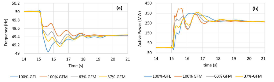
Figure 1 - (a) Frequency, (b) BESS response, in scenarios A to D
- The higher the share of GFM inverters is, the quicker is the overall response of the BESS to the frequency change. This can be attributed to the inertial response of GFM inverters, which is due to the constant phase-angle of its internal voltage source during and immediately after the event.
- With a higher share of inverters being GFM, the frequency nadir is higher, due to a larger inertial response provided by the BESS. The settling frequency, however, is the same in all scenarios since the same droop value is used for all inverters, across all scenarios.
- RoCoF is smaller when larger shares of inverters are in GFM mode (see Figure 2 for a zoomed-in example).
- The response of GFM inverters is immediate, while GFL inverters respond with a delay associated with the required time for measurement, detection (of frequency leaving the dead-band), etc.
- In scenario A, with 100% GFM inverter (the orange curve in Figure 1-(b)), the active power limit of the BESS is reached during the first second after the disturbance. This is mainly because the inertial response provided by all GFM inverters in this scenario (combined with the relatively large size of the contingency), led to an active power injection beyond the BESS’s thermal rating.
Figure 3-(a) and Figure 3-(b) also present the BESS response and frequency dynamics of the grid, respectively, for a fault and trip of a SC. The SC is located in the centre of several large IBRs and plays a key role in providing system strength to that area. Two cases are simulated with all BESS inverters are either GFL or GFM. As seen, even though no active power generation is lost as a result of this contingency, there is a significant temporary frequency drop (to 49.08 Hz) in the case with GFL BESS. This is mainly due to the fault ride-through (FRT) behaviour of the nearby IBRs causing a temporary energy deficit in the grid (see Figure 5 for an example). As seen, the quicker inertial response provided by GFM BESS (as compared to the FFR provided by the GFL BESS) has resulted in around 0.25 Hz increase in the frequency nadir (the red curves in Figure 3).
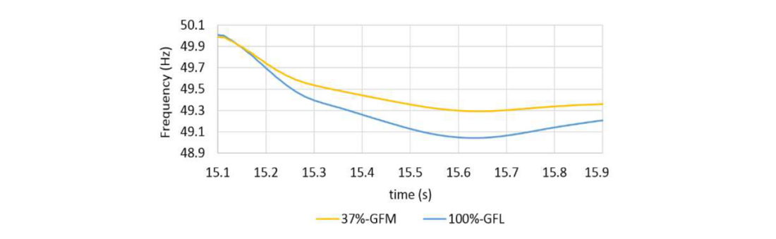
Figure 2 - Frequency traces for scenarios C and D
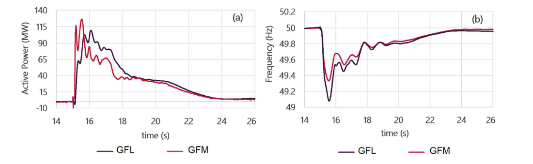
Figure 3 - (a) BESS Response, (b) Frequency, with GFL and GFM, for a SC trip contingency
3. The Role of Inertia Constant of GFM Inverters
As mentioned, VMM is a specific way of implementing GFM control for inverters, in which the dynamics of SGs are modelled in the inverters’ control system. Two main parameters in the VMM control approach are inertia constant (H) and damping constant (D). Unlike SGs, in which the inertia constant is a physical and fixed parameter, in VMM the inertia constant is programable. In other words, VMM allows for adopting very high inertia constants which may not be materialized in reallife SGs of similar MVA rating [17]. In this section, the impact of using different, including a very high, inertia constants for GFM inverters on the frequency response of the grid is investigated. Four scenarios were studied as follows, in all of which a 300 MW BESS is in service, and a 200 MW generation loss contingency is considered:
- Scenario E: GFM BESS with H = 17s
- Scenario F: GFM BESS with H = 9s
- Scenario G: GFM BESS with H = 3s
- Scenario H: GFL BESS
Figure 4-(a) and Figure 4-(b) present the frequency dynamics and BESS responses, respectively, for the above scenarios. The following outlines the key observations:
- The higher the inertia constant of the GFM BESS, the larger the initial active power injected into the system by the BESS. This, however, does not make any significant improvement in the frequency nadir.
- Higher inertia constants have degraded the damping of the system. This can be seen in both frequency and BESS responses (the blue curves). This can be mitigated by adjusting the damping constant, as will be discussed in section 7.
- Even with low inertia constants, GFM BESS leads to higher frequency nadir compared to GFL BESS. This is due to the quicker synthetic inertial response provided by the GFM BESS.
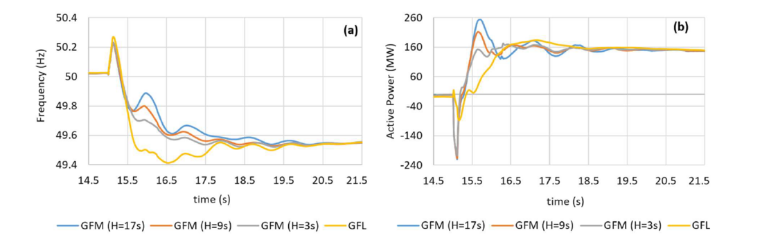
Figure 4 - (a) Frequency, and (b) BESS active power response in scenarios E to H
4. The Role of Fault Current and System Strength Contribution by GFM Inverters
Fault current contribution during the network faults is an important factor in the provision of system strength support to the grid as well as for the correct functioning of protection systems [4]. This requires GFM inverters to be built with sufficient overcurrent capability. Fault current and system strength support provision by GFM inverters can also affect the frequency performance of the grid, in two main ways:
- Through fault current injection during the fault, GFM inverters assist in lifting the voltages and thereby mitigate the temporary drop in active power generation by nearby IBRs. Less power deficit during the fault leads to a smaller frequency drop, although the impact of this might be small.
- Through the provision of system strength, GFM inverters can improve the FRT performance of nearby IBRs and assist them to recover their active power setpoint more quickly and stably after the fault clearance. This can also decrease the temporary energy deficit after the fault and mitigate the frequency drop.
Figure 5-(a) and Figure 5-(b) show the total active power generation by all IBRs and the fault current contribution of the BESS, respectively, for a 200 MW generation loss contingency. Two cases are simulated with all the BESS inverters are either GFL or GFM. As seen, GFM BESS provides a much higher fault current contribution during the fault period and as a result, the momentary drop in active power generation by all IBRs is around 150 MW less than the case with GFL BESS. Less active power deficit during the fault, leads to a slower deceleration of the rotor of SGs which indicates a smaller RoCoF.
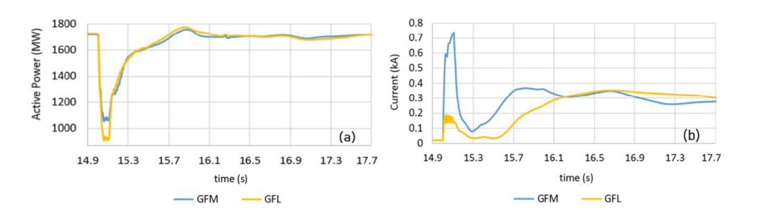
Figure 5 - (a) Total IBR Generation, (b) Fault Current Contribution, with GFM and GFL inverters
5. The Impact of Droop Constant
The longer-term active power responses of both GFL and GFM inverters to frequency deviations are determined by their droop settings. Droop constant determines the active power increase/decrease in response to a specific amount of frequency deviation (usually ~1 Hz, ignoring the frequency deadband). It is important to notice that the inertial response of the GFM inverters is independent of its droop constant and is determined by the value of inertia constant H. In fact, after the initial response of the BESS, governed by its VMM control settings (mainly H constant), the droop control takes over to determine its longer-term response. Figure 6-(a) and Figure 6-(b) show the frequency dynamics and active power responses of the GFM BESS, respectively, to a 200 MW generation loss contingency and with two different droop values. Both cases use the same inertia constant. As seen:
- The inertial response is the same between the two cases, and hence the initial frequency dynamics (including RoCoF) are very similar for both cases.
- After the inertial response, in the case with more aggressive droop (the orange curves) GFM BESS provides more active power. This, increases both frequency nadir and settling frequency, compared to the cases with less aggressive droop (the blue curves).
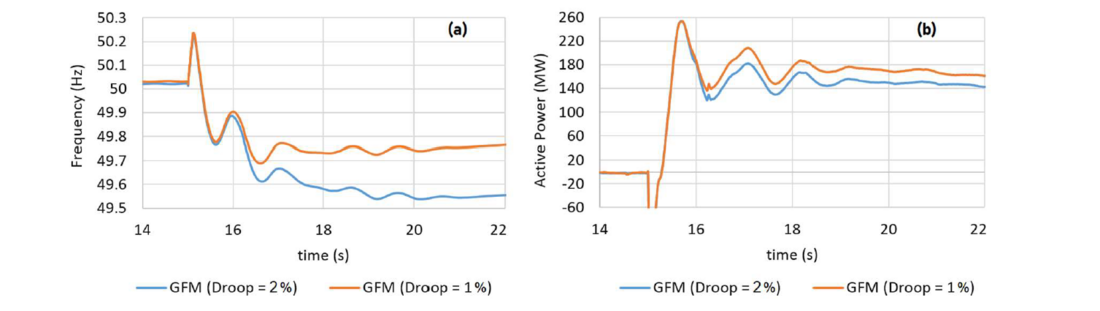
Figure 6 - (a) Frequency and (b) GFM BESS Response, with different droop values and the same inertia constant
As discussed in Section 1, FFR provided by GFL inverters can largely assist with frequency control, however it cannot fully replace the inertial response. This is shown in Figure 7, where the responses of the GFL BESS with two different droop values are compared against the response of the GFM BESS. BESS sizes are the same in all the cases. As observed:
- The use of a more aggressive droop for GFL BESS (the yellow curves) improves the frequency dynamics of the system, however the initial frequency drop is still higher than the case with GFM BESS (which uses a less aggressive droop constant of 2).
- A more aggressive droop cannot mitigate/resolve the delay (~250 ms) in the response of the GFL BESS, as compared to the immediate inertial response of GFM BESS (the blue curve in Figure 7-(b)). Hence, the initial RoCoF is still lower with the GFM BESS.
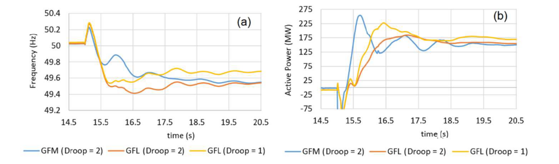
Figure 7 - (a) Frequency, (b) BESS Response, with different droop values for GFL BESS
6. The Impact of Damping Constant
Provision of virtual damping is one of the capabilities of VMM control which is modelled along with the swing equation in the GFM’s control system, through the parameter damping constant (D in MW.s/radian). The damping power component is often calculated through a feedback signal from either virtual speed deviation or its derivate and is negatively fed back into the active power reference of the inverter [19].
To investigate the impact of damping constant on the response of the GFM BESS to a frequency event, four case studies have been simulated, with the results presented in Figure 8. The key findings are as follows:
- Figure 8-(b) shows that in the cases with a higher damping constant (the orange and yellow curves), active power damping is improved compared to the case with a lower damping constant (the black curve).
- Comparing the frequency dynamics of the black and green curves in Figure 8-(a), confirms again that having too large inertia constant does not necessarily improve the frequency dynamics of the system, while it exacerbates the damping performance.
- When using larger inertia constants, the damping constant needs to be also adjusted accordingly to achieve a desired damping behaviour (see the orange curves in Figure 8). Finding the optimal damping constant for each inertia constant, however, is out of the scope of this paper.
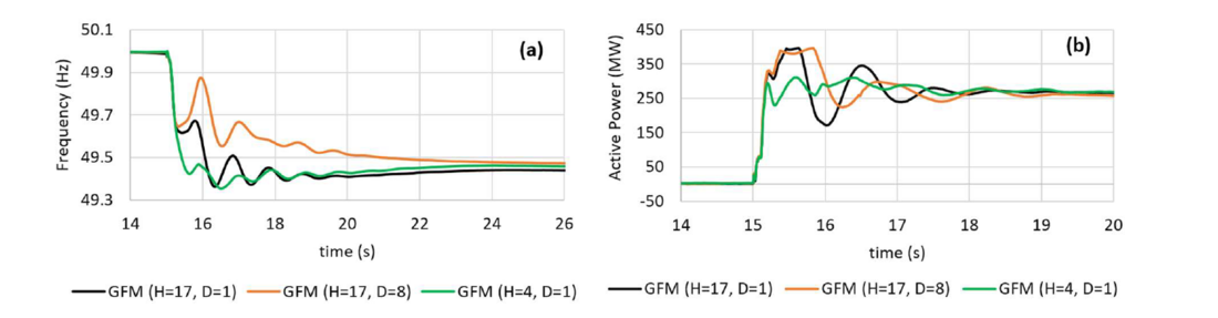
Figure 8 - (a) Frequency, (b) BESS Response, with different inertia and damping constants of GFM inverter
7. Effective Inertia with GFL and GFM BESS
Early methods of estimating the power system inertia only include the known contributions from large transmission-connected SGs. This method, however, can only set the lower bound of total system inertia, since it ignores the inertia contribution from smaller distributed-connected generators, synchronous and induction motors, as well as the synthetic inertia provided by some IBRs. For instance, in Great Britain, demand-side inertia was estimated to vary between 17% to 25% of the total system inertia [22]. Effective inertia is a more accurate metric to estimate the system’s total inertia. It defines the relationship between the active power imbalance upon a contingency and the RoCoF. The method has been used for estimating the total inertia of a region of the WECC grid [23].
Effective inertia estimation methods are mostly based on linearized swing equation, as per eq. (1) [24]:
(1)
where EISYS is grid’s effective inertia (MWs), ?n is the nominal frequency (Hz), ΔP is the size of contingency (MW), and ?Δ?/?? is an estimate of the RoCoF (Hz/s) at the onset of the contingency. RoCoF should be measured before the activation of any FFR and governor responses, to exclude their impacts from the assessment [25]. In this section, the impact of synthetic inertia provided by GFM inverters on the grid’s effective inertia is assessed and compared against that of FFR provided by GFL inverters.
Two scenarios were studied, one with GFL BESS and one with GFM BESS (both 300 MW). In both scenarios, 4400 MW.s of physical inertia is available through synchronous machines. A 40 MW load trip contingency is applied in both scenarios. Figure 9 shows the frequency traces for both scenarios. The RoCoF values are also shown in the figure for each scenario, which are calculated before the frequency exists the dead-band of ±0.015Hz in the GFL BESS scenario. The effective inertia values calculated for each scenario using eq. (1) are as follows:
- 4500 MWs in the GFL BESS scenario, which is very close to the collective physical inertia available through the synchronous machines in the region (~4400 MWs). This verifies the accuracy of the results and also indicates the limited inertia contribution by GFL BESS.
- 6700 MWs in the GFM BESS scenario, which signifies the considerable impact of GFM BESS on the grid’s effective inertia.
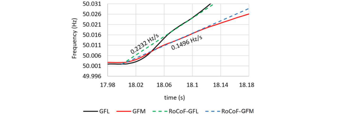
Figure 9 - Frequency dynamics for a 40 MW load loss, with GFL BESS and GFM BESS
These results indicate that the amount of energy exchanged with the grid immediately after a frequency event is considerably larger in the GFM BESS scenario, similar to the inertial response of SGs.
8. Conclusion
This paper investigates the impacts of inertial response provided by a GFM inverter on the power system frequency stability. Several scenarios are studied to investigate and compare the responses of GFM and GFL inverters to frequency disturbances, and to study the impact of different parameters of GFM inverter on its frequency response. Results indicate that GFM inverters can make a significant improvement in the frequency stability of the grid mainly through their immediate synthetic inertial response to the frequency disturbances. It was shown that using an aggressive droop in the FFR of a GFL inverter cannot fully replace the inertial response provided by a GFM inverter, due to the inherent delay in the GFL inverter’s response. Results also demonstrate that using large inertia constants in a GFM inverter do not necessarily improve the frequency performance of the grid, while it might deteriorate the damping performance. To prevent this, damping constant needs to be adjusted along with the inertia constant. Fault current contribution and system strength support of GFM inverters are also shown to have an impact on improving the grid’s frequency stability, by helping nearby IBRs ride through the faults more smoothly and quickly. Finally, through calculating the effective inertia of the grid, it was shown that inertia contribution of GFL technology is quite limited, compared to the significant inertia contribution by GFM inverters. The time delay inherent to the FFR would require sufficient effective inertia to be online to limit the RoCoF, until the FFR and other slower frequency responses are initiated.
References
- IEEE, “Renewables in Australia”, IEEE Power & Energy Magazine, Vol. 19, n. 5, October 2021
- AEMO, “Transfer Limit Advice, System Strength in SA and Victoria”, Australian Energy Market Operator, July 2021
- Matevosyan, Julia, et al. "Grid-forming inverters: Are they the key for high renewable penetration?." IEEE Power and Energy magazine 17.6 (2019): 89-98.
- AEMO, “Application of Advanced Grid-scale Inverters in the NEM – white paper”, Australian Energy Market Operator, August 2021.
- Babak Badrzadeh, “Australian Experience with Grid Forming Inverters”, Energy Systems Integration Group (ESIG), March 2021.
- Stephen Sproul, Stanislav Cherevatskiy, Hugo Klingenberg, “Grid Forming Energy Storage: Provides Virtual Inertia, Interconnects Renewables and Unlocks Revenue”, Hitachi ABB, July 2020.
- NERC, "Fast frequency response concepts and bulk power system reliability needs." NERC Inverter- Based Resource Performance Task Force (IRPTF), March 2020.
- AEMO, "Fast frequency response in the NEM", Australian Energy Market Operator, 2017.
- A. Isaacs, C. Hardt, S. Walinga, E. Quitmann, D. Ramasubramanian, T. Lin, "Grid Forming Technology: Current Applications and Future Considerations", IEEE PES General Meeting, Panel session, July 2021.
- Andrew Isaacs, “Grid-Forming Definition”, Energy Systems Integration Group (ESIG), March 2021.
- Julia Matevosyan, “Survey of Grid Forming Inverter Applications”, Energy Systems Integration Group (ESIG), June 2021.
- Cherevatskiy, S., Zabihi, S., et al. "A 30MW grid forming BESS boosting reliability in South Australia and providing market services on the national electricity market." 18th International Wind Integration Workshop, Dublin. 2019.
- Tesla, “Hornsdale Power Reserve Virtual Machine Mode Model Dual Inverter Trial Report”, Tesla Energy Products, July 2021.
- H.-P. Beck and R. Hesse, “Virtual Synchronous Machine,” in Proc. 9th Int. Conf. Elect. Power Qual. Utilization, Barcelona, Spain, 2007, pp. 1–6.
- Tim Green, Yunjie Gu, Yitong Li, “Research Landscape for Grid Forming Inverters”, Energy Systems Integration Group (ESIG), March 2021.
- Hitachi ABB, “e-mesh PowerStore high-power grid-forming inverters - Unlocking new revenue and stabilizing large electric grids with energy storage”, ABB Power Grids, 2021.
- Tayyebi, Ali, et al. "Frequency stability of synchronous machines and grid-forming power converters." IEEE Journal of Emerging and Selected Topics in Power Electronics 8.2 (2020): 1004-1018.
- Tuckey, Andrew, and Simon Round. "Practical application of a complete virtual synchronous generator control method for microgrid and grid-edge applications." 2018 IEEE 19th Workshop on Control and Modeling for Power Electronics (COMPEL). IEEE, 2018.
- Meng, Xin, Jinjun Liu, and Zeng Liu. "A generalized droop control for grid-supporting inverter based on comparison between traditional droop control and virtual synchronous generator control." IEEE Transactions on Power Electronics 34.6 (2018): 5416-5438.
- Poolla, Bala Kameshwar, Dominic Groß, and Florian Dörfler. "Placement and implementation of gridforming and grid-following virtual inertia and fast frequency response." IEEE Transactions on Power Systems, 34.4 (2019): 3035-3046.
- Babak Badrzadeh, Z. Emin, Emil Hillberg, David Jacobson, Lukasz H. Kocewiak, G. Lietz, Marta val Escudero, “The Need for Enhanced Power System Modelling Techniques and Simulation Tools”, CIGRE Science & Engineering Journal, February 2020.
- Y. Bian, H. Wyman, F. Li, R. Bhakar, S. Mishra, N. P. Padhy, “Demand Side Contributions for System Inertia in the Great Britain Power System”, IEEE Transactions on Power Systems, vol. 33, no. 44, pp. 3521-3530, July 2018.
- G. Chavan, M. Weiss, A. Chakrabortty, S. Bhattacharya, A. Salazar, and F. H. Ashrafi, “Identification and predictive analysis of a multi-areaWECC power system model using synchrophasors,” IEEE Trans. Smart Grid, vol. 8, no. 4, pp. 1977–1986, Jul. 2017.
- Kaur Tuttelberg, Jako Kilter, Douglas Wilson, Kjetil Uhlen, “Estimation of Power System Inertia From Ambient Wide Area Measurements”, IEEE Trans. on Power Systems, vol. 33, no. 6, pp. 7249–7257, November 2018.
- P. M. Ashton, C. S. Saunders, G. A. Taylor, A. M. Carter, and M. E. Bradley, “Inertia estimation of the GB power system using synchrophasor measurements”, IEEE Transactions on Power Systems, vol. 30, no. 2, pp.701–709, March 2015.