Enhancing deliverability of reserves through market price signals
Authors
Pradip KUMAR, Matt MUSTO, Kanchan UPADHYAY - NYISO, United States

Summary
Operating reserves provide the necessary back-up supply to respond to real-time contingency scenarios and are critical to ensure grid reliability. Currently, the operating reserve requirements in New York are based upon the output of large baseload generation at the balancing area level. The locational requirements are based on the reliability criteria to ensure appropriate distribution to ensure deliverability. These requirements are held constant throughout the 24 hours and 365 days of the year. The enactment of the Climate Leadership and Community Protection Act (CLCPA) in New York State in 2019 set ambitious targets for the state, including attaining 70% renewable power generation by 2030 and achieving a zero-emission electric system by 2040. Evolving grid with substantial share of variable renewables poses a challenge to using static predetermined operating reserve requirements. There is a need for increasing existing reserves available on grid to compensate for variable resources. Owing to the variable nature of these resources, going into the future grid, the largest generation may be an offshore wind unit, which is not expected to operate at the same level of throughput during all hours of the day. It is critical for New York Independent System Operator (NYISO) to develop an effective and efficient mechanism to hold sufficient operating reserves to compensate for intermittent renewables and uncertain net load. Enhancing deliverability of reserves through efficient market signals is a key component of a series of changes contemplated by the NYISO.
This paper describes how dynamic reserves scheduling and pricing mechanisms can be enhanced to ensure that reserves are procured where they are most needed on the grid. This paper goes into detail on the nodal pricing for reserves, impact of the nodal reserves model on energy price formation and how to develop appropriate locational marginal prices in this model.
Keywords
Dynamic Reserves, LBMP (Location Based Marginal Prices), LMORP (Locational Marginal Operating Reserves Prices), NYCA (New York Control Area), Operating Reserve Requirements, Price Formation, Variable Energy Sources1. Attracting the correct grid reliability resources through wholesale markets
Maintaining a reliable energy system requires that enough power generating capacity is installed system-wide to meet projected electricity demand and reliability requirements. For the past 25 years, competitive wholesale electricity markets in New York have supported the reliable, efficient operation of the grid. An added benefit of wholesale electricity markets is that competition among resources rewards economic efficiency. Historically, this has resulted in cleaner and more efficient supply coming onto the grid and displacing older, less efficient supply.
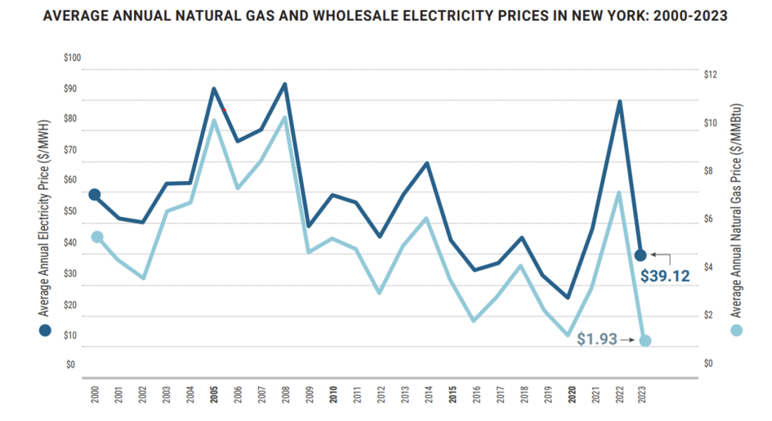
Figure 1 - Correlation of natural gas prices to wholesale electricity price in New York
Wholesale electricity markets use price signals to attract and retain enough supply in the most beneficial locations on the system to provide needed reliability services. Today’s grid consists largely of dispatchable resources that respond quickly to system needs. The costs to procure adequate capacity for projected peak demand levels and to produce electricity in the precise quantities needed by the grid in real-time are all included within the cost of wholesale electricity, but the NYISO manages a separate market for each to support their different purposes.
Transitioning to the clean energy grid of the future will require unprecedented investment in new supply resources. Competitive markets support and encourage continuous gains in efficiency and innovation. Inefficient producers are replaced by new, cost-effective, and cleaner technology. Market-based price signals are transparent and stimulate necessary infrastructure investment to meet renewable and decarbonization goals, energy conservation, and demand response.
In a clean energy grid of the future, a premium attribute of energy supply will be its flexibility. Market innovations are necessary that will attract flexible resources that perform when needed and reward those resources that can support balancing grid supply and demand. With ever-increasing intermittency, extreme weather, and demand from electrification and economic development, the economic force of markets is essential for maintaining reliability.
2. The New York Electricity Market
The wholesale energy market in New York encompasses both a Day-Ahead and a Real-Time market for electricity. The financially binding Day-Ahead market enables advanced scheduling for generators requiring notice, fostering adherence to operating schedules. This financial commitment also incentivizes all generators to perform as scheduled. Given the dynamic nature of anticipated load, available generation, and system conditions, the NYISO operates a Real-Time market to efficiently balance system changes as they occur.
Operating reserves ensure sufficient supply to meet changing conditions in real-time, such as unplanned generator or transmission outages. Historically this need was solved by identifying fixed, system-wide reserve requirements. As renewable capacity grows and supply to the grid is more susceptible to changing weather conditions, establishing dynamic reserve requirements will support renewable energy integration by more accurately accounting for uncertainty and procuring this additional reserve at the lowest cost to consumers.
3. Dynamic Reserves Approach in Establishing Reserve Requirements
The variable nature of sustainable energy sources such as wind and solar, requires reserves to be adjusted based on the level of intermittent generation and existing system conditions. Several reports and technical papers [1] [2] [3] indicate a growing interest in setting reserves dynamically in the US Regional Transmission Operator (RTO)/ Independent System Operator (ISO) administered markets [4]. NYISO has developed a proposal for setting dynamic reserves which has been endorsed by its stakeholders in December 2024 [5].
The NYISO’s dynamic reserves proposal introduces an endogenous approach to determining reserve requirements, incorporating the loss of the largest energy-producing generator or the loss of transmission element into the optimization process. This dynamic method establishes the reserve requirement for each interval of both Day-Ahead and Real-Time Market operations. In contrast, NYISO's current static requirements do not account for the real-time potential of the largest source contingency changing, based on actual generation output or system topology. This static approach may lead to over-procurement of reserves during certain hours and under-procurement during others since a fixed quantity of reserves is procured throughout the day. While this conservative approach ensures reliability by meeting or exceeding the loss of energy due to the largest contingency, it proves to be expensive when the largest unit on the grid is a renewable energy source like wind or solar.
3.1. Endogenizing Reserve Procurement Criteria within the NYISO’s Market Model
The Security Constraint Unit Commitment (SCUC) and Security Constraint Economic Dispatch (SCED) formulations within the New York Independent System Operator (NYISO) Market Management System (MMS) are designed to minimize total production costs, encompassing both energy and ancillary service procurements, while ensuring that load and transmission security constraints are met. The NYISO-controlled transmission system, which includes the majority of the 100kV and higher lines within the New York Control Area (NYCA), is operated according to Normal transfer criteria. This criterion is satisfied when the actual loading on a transmission facility does not exceed its associated Normal rating, and when a single (N-1) contingency does not cause any facility to exceed its Long-Term Emergency (LTE) rating.
Operating reserves are procured to ensure that sufficient resources are available to maintain system reliability in the event of a real-time contingency. Under a static reserve requirements framework, these reserves are typically based on the output of the largest base-load units [6]. However, this approach may not be effective in situations where the largest contingencies are large variable resources, such as Offshore Wind plants, whose output fluctuates throughout the evaluation period. To address this, the concept of Dynamic Reserve requirements are introduced, which integrates reserve procurement criteria within the NYISO’s market model. This dynamic framework calculates reserve requirements for each evaluation interval based on the total schedules of the largest units. Table 1 illustrates the Dynamic Reserve calculation criteria for system-wide reserve requirements, highlighting the connection to the Reliability Rule that currently forms the basis for static requirements.
| Current Static Value | Reliability Rule | Dynamic Reserve calculation criteria | |
|---|---|---|---|
| 10-Minute Spinning Reserves | 655 MW | 10-Minute spinning reserve is equal to at least half of the 10- minute total reserve. | Equal to 1/2 times the largest schedule among internal generators or external proxies for a given period. The largest schedule is formulated as the combined energy, regulation and operating reserves schedule. |
| 10-Minute Total Reserves | 1310 MW | 10-Minute total reserve is equal to the operating capability loss caused by the most severe contingency under normal transfer conditions. | Equal to the largest schedule among internal generators or external proxies for a given period. The largest schedule is formulated as the combined energy, regulation and operating reserves schedule. |
| 30-Minute Total Reserves | 2620 MW | 30-Minute total reserve is equal to two times the 10-minute reserve necessary to replace the operating capability loss caused by the most severe contingency under normal transfer conditions. | Equal to the sum of largest schedule and second largest schedule among internal generators or external proxies for a given period. The largest schedule is formulated as the combined energy, regulation and operating reserves schedule. |
Granular locational reserve requirements are founded on the principle of restoring a transmission circuit to its appropriate operating limits following a contingency. Offline studies are conducted to determine the appropriate static reserve requirements within a designated Reserve Area. Since these requirements are static, they are often established using conservative estimates of line loadings.
The NYISO’s Dynamic Reserves design [8], seeks to minimize costs by balancing the procurement of reserves with system prepositioning, thereby reducing overall "insurance" expenses. The unified nodal reserve design incorporates reserve criteria into the optimization model, enabling the system to achieve greater flexibility and transparency. This approach allows the optimization engine to make cost-effective decisions between energy and reserve scheduling, ensuring the transmission system meets reliability criteria while serving load efficiently.
Reserve criteria vary by reserve type. For instance, 10Total reserves secure the transmission facility to the Long-Term Emergency (LTE) limit in response to the loss of either a single transmission element or a single generation element. In contrast, 30Total reserves ensure system security to the Normal limit for the loss of one transmission or generation element, or to the Long-Term Emergency limit for the simultaneous loss of two transmission elements, two generation elements, or a combination of one transmission and one generation element.
3.2. Unified Nodal Reserve Model with Energy Scheduling
Endogenizing the locational reserve criteria within the market model integrates reserve flows with post-contingency energy flows. This approach uses shift factors to assess the impact of energy and reserve schedules from various generators on secured transmission elements. The foundational framework of the SCUC (Security-Constrained Unit Commitment) and SCED (Security-Constrained Economic Dispatch) constraints, incorporating dynamic reserve criteria, is outlined below.
(1)
Equation 1 is the objective function of a standard economic dispatch model that minimizes the total production cost of the system by considering the cost of each unit i in time period t to produce energy Gmwi,t and the cost
associated with holding capacity to offer reserves Gresi,t
Subject to:
Equation 2 is the energy balance constraint that ensures that the energy produced by the generators i, meet the demand j, in each interval t. The shadow price of the constraint defined as is the marginal cost of the next incremental MW of energy produced
(3)
Equation 3 is a generation capacity check that ensures that the energy and reserves scheduled on a unit do not exceed the maximum capacity of the unit i in interval t
Equation 4 is the total of all spinning reserves from units that meets or exceeds the 10 minute spinning reserve requirement which is half of the largest generator schedule in interval t. The shadow price of the constraint defined as is the marginal cost of the next incremental MW of 10-minute spinning reserve capacity procured
Equation 5 is the total of all spinning and non-spinning reserves from units that meets or exceeds the 10-minute total reserve requirement which is the largest generator schedule in interval t. The shadow price of the constraint defined as is the marginal cost of the next incremental MW of 10-minute total reserve capacity procured
Equation 6 is the total of all spinning and non-spinning reserves from units that meets or exceeds the 30-minute total reserve requirement which is the sum of the largest and second largest generator schedules in interval t. The shadow price of the constraint defined as is the marginal cost of the next incremental MW of 30-minute total reserve capacity procured
Equation 7 is the constraint for each secured transmission element under different contingency scenarios, that ensures the flow is less than the appropriate limit for the secured transmission element. Flow is calculated as the sum of energy schedules across generators times their sensitivity/shift factor and sum of zonal load times zonal sensitivity/shift factor
TC in limittc,t is the set of :
- Base case transmission constraints i.e. securing the flow on transmission elements to Normal limits for base case scenarios
- Contingency case transmission constraints i.e. securing the flow on transmission elements to Emergency limits under different contingency scenarios
The shadow price of the constraint defined as contributes to the congestion component of Locational Marginal Price (LMP) at a location.
Generic Formulation of Dynamic Reserve constraint for “loss of transmission element”:
Equation 8 is the post-contingency flow for the loss of a transmission element that is calculated as the sum of energy schedules and reserve schedules
across generators times their sensitivity/shift factor and sum of zonal load times zonal sensitivity/shift factor
for respective constraint. The shadow cost of the constraint
impacts the nodal price of energy and reserves as shown in later sections.
Generic Formulation of Dynamic Reserve constraint for “loss of generation element” is:
Equation 9 is the post-contingency flow for the loss of generator m that is calculated as the sum of energy schedules and reserve schedules
across generators (except generator m) times their sensitivity/shift factor and sum of zonal load times zonal sensitivity/ shift factor
for each constraint. The shadow cost of the constraint
impacts the nodal price of energy and reserves as shown in later sections.
3.3. Reserves price formation with nodal reserve markets
Dynamic reserve design proposal will result in a shift from reserve prices at reserve area level to nodal prices, more accurately reflecting a resource’s ability in supporting reliability. These nodal reserve prices, referred to as Locational Marginal Operating Reserve Price (LMORP) will be calculated for all reserve product types and would reflect the incremental value of the operating reserve product at the pricing node. LMORPs at each node will comprise of two elements:
- System marginal operating reserve product price: This is the shadow price of the system-wide reserve constraint for reserve product r
as defined in equations (4) – (6). All the reserve providers located within the NY control area can meet NYCA reserve requirements and their LMORP will reflect the shadow prices of NYCA reserve constraints
- Shadow prices for Locational dynamic reserve constraints: These are the shadow prices associated with locational dynamic constraints for different contingency scenarios (
and
) as described in equations (8) and (9). Each reserve providers ability to relieve the locational reserve constraints is based on their shift factor to the respective constraint. This component of LMORP is calculated as the sum product of the shift factor of reserve provider times the shadow price of respective constraint.
LMORPr for reserve product r at generator i node can be calculated as: [1]
The price calculated for each reserve production type r considers all the constraints (set R = 10Spin, 10Total, 30Total) the product can help, as such reserve price cascading across product types is inherent in LMORP calculations.
- • 10Spin product type can solve 10Spin, 10Total and 30Total NYCA and Locational dynamic reserve constraints, therefore the LMORPi,r=10Spin,t shall include applicable NYCA and locational constraints shadow prices.
- • 10Total product type can solve 10Total and 30Total NYCA and Locational dynamic reserve constraints, therefore the LMORPi,r=10Spin,t shall include applicable NYCA and locational constraints shadow prices.
- • 30Total product type can only solve 30Total NYCA and Locational dynamic reserve constraints, therefore the LMORPi,r=10Spin,t shall include applicable NYCA and locational constraints shadow prices.
3.4. Energy price formation with nodal reserve markets
In NYISO’s electricity markets, energy and reserves are co-optimized ensuring that a generating resource is indifferent to providing energy or reserves. As such, reserve prices currently impact Locational Based Marginal Prices (LBMPs) given the unit capacity level constraints and co-optimization as represented in Equation (3). Under the dynamic reserves framework, the impact of reserve requirements constraint on energy prices is more direct and prominent. Post-contingency flow evaluation for locational dynamic reserve requirements is based on the flow created by both energy and reserve schedules. This means that in addition to the constraints that impact the LBMPs today, there are additional set of locational reserve constraints that need to be accounted for when calculating energy prices.
Constraints that impact the energy prices include:
- Power Balance constraint (shadow price
)
- • Transmission Constraints (shadow price
)
- • Reserve Constraints (shadow price
Ignoring losses, the LBMP at generator i node shall comprise of :
- System Lambda,
- Transmission congestion component: Transmission congestion component is calculated the sum product of the shift factor of energy providers times the shadow price of respective transmission constraint.
- Reserve congestion component: Reserve congestion component is calculated the sum product of the shift factor of energy providers times the shadow price of respective locational reserve constraint.
Formulaically, LBMP at generator i node can be calculated as:[2]
3.5. Annotation
The variables used in the equations in this paper is annotated below for reference.
Index
- i:generator
- j:load bus
- t:dispatch interval
- tc:transmission constraints, a pair of contingency type and transmission facility
- drtc:dynamic reserves constraints, a pair of contingency type and transmission facility
- r:reserve categories
Set
- I:set of generators
- J:set of load buses
- T:set of dispatch intervals
- TC:set of transmission constraints
- DRTC:set of dynamic reserve constraints
- R:set of reserve categories {′10Spin′,′10Total′,′30Total′}
Parameters
:energy bid for gen ?
:reserve bid for gen ?
- gmxi,t:upper operating limit for gen ?
- fldj,t:forecast load at load bus j
- limittc,t:line limit for transmission constraint tc
- limitdrtc,t:line limit for reserve constraint drtc
- sftc,i,t:shift factor of generator i for transmission constraint tc
- sftc,j,t:shift factor at load bus j for transmission constraint tc
- sfdrtc,i,t:shift factor of generator i for reserve constraint drtc
- sfdrt,j,t:shift factor at load bus j for reserve constraint drtc
Variables
- Gmwi,t:energy schedules for generator ?
- Gresi,r,t:reserve schedules for generator ? in reserve catory r
- ldj,t:load schedule at bus j
:largest generator schedule (energy+reserves+regulation) in interval t
:sum of largest and second largest generator schedule (energy+reserves+regulation) in interval t
4. Benefits of Nodal Dynamic Reserves design
The dynamic reserves design represents a significant stride toward achieving the New York state policy mandates. This design aligns with the criteria used to meet static reserve requirements today but anticipates the variability introduced by the increasing deployment of renewables in the coming years. The key benefits of this design are as follows:
- Dynamically securing Reserves for Largest Source contingencies in the NYCA will facilitate the incorporation of large variable energy resources, such as Offshore Wind Power plants
- Reserve requirements that are based on system conditions will allow better reflection of reliability costs in markets
- Locational Reserve requirements endogenizing reliability criteria will allow optimal tradeoffs between energy and reserves to secure loadings on transmission circuits/interfaces to Normal Operating criteria within 15 minutes following a contingency.
- Utilization of shift factors provides for more accurate assessment of resources impact to ensure reliability. Also facilitate calculation of nodal reserve prices or LMORP to create better market incentives
- Securing reserves to NYISO’s DAM Forecast Load supports reliable operations by assigning DAM schedules to needed resources
5. Implementation challenges
The transition from pre-calculated Operating reserve requirements to a dynamic determination offer improvements in reliability and market efficiency but also presents few challenges. The implementation of the design will increase the number of security constraints in the market model presenting a risk to computational performance. NYISO is actively working to address this challenge by exploring innovative mathematical solutions such as Redundant Constraint Filtering algorithm to reduce the number of additional security constraints and thereby improve computational performance. In addition to significant enhancements to the market model, dynamic reserves will also have implications across multiple facets of markets such as settlements, market validation, public posting and more making the implementation a resource intensive and time-consuming endeavour. The transition also introduces a fundamental change in the construct of operating reserves and requires training and experience on the grid operation side to operate in the new paradigm.
Conclusion
This paper introduces the concept of nodal reserve pricing, designed to enhance the deliverability of reserves and establish price signals that incentivize reserve allocation where it is most needed on the grid. As system conditions fluctuate throughout the day, energy and reserve prices dynamically adjust to reflect the reliability requirements necessary for maintaining grid stability.
Moreover, this framework prepares the grid for a future in which the largest energy-producing resource is no longer a traditional baseload unit, such as a nuclear facility, but rather a variable renewable resource, like wind, whose output can fluctuate significantly over time. The proposed approach also accounts for the fact that the largest energy-producing unit may not be a fixed resource. Instead, it dynamically identifies the largest unit at any given moment, adjusting reserve requirements accordingly.
While this methodology effectively integrates dynamic reserve requirements to support system reliability, it also introduces a more complex pricing mechanism and presents operational challenges like reserve requirements changing significantly in a short duration of time. The NYISO is actively addressing these challenges to ensure the successful implementation of this concept.
References
- Y. Sun, J. Nelson, J. Stevens, A. Au, V. Venugopal, C. Gulian, S. Kasina, P. O'Neill, M. Yuan and A. Olson, “Machine Learning Derived Dynamic Operating Reserve Requirements in High-Renewable Power Systems,” DOE OSTI Report, May 18, 2022.
- K. Hedman, M. Zhang, M. Ilic, J. Lyon, F. Want, C. Li and J. Prada, “Markets for Ancillary Services in the Presence of Stochastic Resources,” PSERC Report, September 2016.
- M. Ilic and D. Zhao, “Dynamic Reserves for Managing Wind Power,” in 2023 IEEE Power & Energy Society General Meeting (PESGM), Orlando, FL, USA, July 2023.
- Mid Independent System Operator (MISO), “Short - Term Reserves Conceptual Design,” October 3, 2019.
- New York ISO, “Dynamic Reserves Market Design,” in Business Issue Committee Meeting, December 11, 2024.
- NYISO, “NYISO Locational Reserve Requirements,” 29 January 2025. [Online].
- New York State Reliability Council, “Reliability Rules & Compliance Manual”, Version 46, June 10, 2022. Available online.
- P. Kumar, M. Musto, N. Gilbraith, R. Mukerji, M. Desocio “Dynamic Procurement of reserves in New York Electricity Markets”, 2024 CIGRE Paris Session, Ref C5-10467-2024.
- [1] If loss of generator m is a binding Dynamic Reserve constraint, then the shadow price of the “LossG” constraint will not be accounted for in calculation of LMORP for generator m. In the formulation of dynamic reserve constraint for loss of generation m in equation (9), generator m is excluded from the summation on the LHS of the equation.
- [2] If loss of generator m is a binding Dynamic Reserve constraint, then the shadow price of the “LossG” constraint will not be accounted for in calculation of LBMP for generator m. In the formulation of dynamic reserve constraint for loss of generation m in equation (9), generator m is excluded from the summation on the LHS of the equation.