Active Energy Metering in Synchronous Condensers
Author
Graeme VERTIGAN - Australia

Summary
In recent years synchronous generation has progressively been displaced by inverter-based sources from wind and solar farms, which has resulted in a steady decline in transmission fault levels. Synchronous condensers have resurfaced as a way of restoring these, as well as providing voltage support by exporting reactive power to the network when the voltage is low and importing it when the latter becomes high. Because of this, synchronous condensers are frequently associated with renewable generation, especially when it is coupled to weak parts of the transmission system.
Synchronous condensers consume between 2 and 3% of their nameplate rating as active power and when supporting the local bus, operate at very low power factors for much of the time. However small, the running energy supplied by the network is by no means negligible, and must be accurately metered and paid for. This paper describes a little-known phenomenon with energy metering at elevated potentials, whereby a small quantity of active energy cannot be accurately measured against a large quantity of reactive energy. This makes the task of metering the running energy of a synchronous condenser much more difficult and means that a conventional metering installation cannot be used for this purpose.
Keywords
Field excitation, meter uncertainty, overall error, power factor, synchronous condenser1. Energy Meter Errors
Modern energy meters are capable of accurately recording active and reactive energy within the range of power factors that are normally encountered by customer loads. This information is recorded in meter registers which segregate the active and reactive energy imported or exported throughout a metering interval. Metering intervals are typically 0.5h (or sometimes 0.25h) in length and are synchronized to the local time zone.
Customer consumption includes loads with inductive (lagging) power factors from 0.5, through to capacitive (leading) power factors around 0.8. The active error limits for this range are defined in standard IEC62053.22 and appear in Table 1. Here it can be seen that both 0.5S and 0.2S class meters operate best at unity power factors, where the error limits define the class of these meters.
| Value of current | Power factor | Percentage error limits for meters of class: | |
|---|---|---|---|
| 0.2S Class | 0.5S Class | ||
0.01In ≤ I ≤ 0.05In | 1 | ±0.4 | ±1.0 |
0.05In ≤ I ≤ Imax | 1 | ±0.2 | ±0.5 |
0.02In ≤ I ≤ 0.1In | 0.5 inductive | ±0.5 | ±1.0 |
0.1In ≤ I ≤ Imax | 0.5 inductive | ±0.3 | ±0.6 |
When specially requested | 0.25 inductive | ±0.5 | ±1.0 |
If the range of power factors becomes a little wider, from 0.25 inductive to 0.5 capacitive, as shown in the last line of Table 1, the permitted error limits become considerably greater. This is necessary, because as the power factor becomes smaller, the meter’s ability to accurately measure the active energy decreases. What the standard does not show is how poorly energy meters perform when measuring a small quantity of active energy against a large quantity of reactive energy, i.e., when operating at very low power factors.
2. Metering Uncertainties
Uncertainty is a numerical representation of how much doubt exists that a measurement is correct. If the uncertainty is small, then we can have a high degree of confidence that a measurement is likely to be correct. If it is large, then so is the degree of doubt associated with that measurement. Generally speaking, a wide tolerance associated with a measurement implies that there is also likely to be a relatively large level of uncertainty.
The parameter which has most bearing on the uncertainty of an energy measurement is the power factor at which it is made. The meter uncertainty associated with active energy measurement is proportional to the reciprocal of the power actor, i.e., 1/(pf). This means that at unity power factors, the uncertainty takes on its lowest value, but as the power factor decreases, the uncertainty also increases, and at very low power factors it becomes very large indeed. (The converse is true for reactive energy measurements, where the uncertainty is proportional to 1/Sin(φ), where φ is the effective phase angle of the load. Therefore, reactive measurements are most accurate at zero power factor.)
In practice, the uncertainty of energy measurement really depends on the meter in question; some meters simply perform better than others. Unfortunately, this situation is compounded when current and voltage transformers are included in a metering installation. Of course both are necessary for high voltage measurements, and both introduce magnitude and phase errors into the data delivered to the meter. So even if the meter were perfect, the use of instrument transformers will still result in energy measurements that contain a degree of error.
3. Overall Error or Total Error
The performance of an entire metering installation, including instrument transformers as well as the meter itself, is quantified in a figure of merit known as the Overall Error (OE), or sometimes the Total Error. The OE for active power is defined in equation (1).
(1)
Where: Pm = the power measured by the metering installation under test, and
Pc = the correct power recorded by an ideal metering installation, (i.e. one with no inherent errors)
Therefore, positive Overall Error values indicate an over-reading installation, while negative values indicate an under-reading one. It is also possible to express the OE per phase, in terms of the instrument transformer errors and the phase angle of the circuit concerned, as expressed in equation (2).
(2)
Here β is the phase error associated with the current transformer, γ is the phase error associated with the voltage transformer, (usually expressed in Centi-radians (Crad), or sometimes in minutes of arc), ev and ei are the VT & CT magnitude errors, (expressed in percent). Finally, φ is the load phase angle, that by which the current lags the voltage. Both β and γ are small angles, typically less than 0.2Crad, and when resistive burdens are applied to the instrument transformers, (as is normally the case), β is positive and γ is negative, so unfortunately the magnitudes of these angles tend to add in the sine term above. The magnitude errors ev and ei are also small, usually less than 0.5%.
The Overall Error ε, expressed in equation (2) corresponds to just one phase, therefore in a three-element metering installation there will be three ε values. These must be averaged to generate the error result for the entire installation, since in a well-balanced load, the same quantity of energy will be delivered by each phase. Equation (2) also assumes that the meter error is zero, and since this won’t normally be the case, the meter error must be added to this average to achieve the complete Overall Error result for the entire installation. The meter error is defined in a similar fashion to equation (1), and it applies to the total energy recorded across all three phases.
At power factors close unity, the Overall Error is approximately the sum of the instrument transformer magnitude errors, plus the meter error, which usually results in a value around 0.5%. However, as the power factor falls, the tan(φ) sin( β-γ) term in equation (2) becomes larger, slowly at first, but as the power factor falls below 0.1, it begins to increase rapidly. Therefore, for phase angles close to 90 degrees the Overall Error of the installation can easily exceed 100%. The phase errors associated with the instrument transformers together with the load phase angle, are responsible for the poor Overall Error results that occur at low power factors.
This effect is illustrated in Figure 1, which shows how the active Overall Error typically changes with variations in the load power factor. For power factors around unity the Overall Error is acceptably low, however at power factors typical of synchronous condenser operation, (≈ 0.01), the Overall Error can easily exceed 100%.
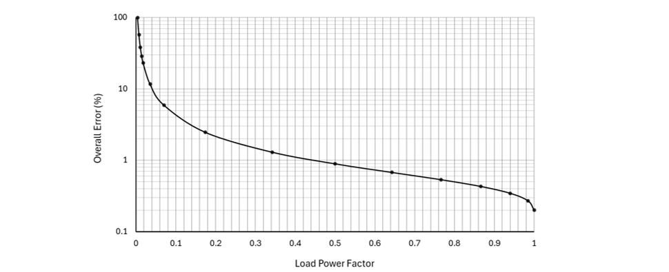
Figure 1 - Typical variation in Overall Error with falling load power factor
By way of example, Figure 2 shows the power recorded in a 1pu resistive load metered along with a variable reactive component, over a range of power factors between 0 and 1. Although the active load remained constant throughout the measurement process, as the reactive load increased, the meter perceived that the former had increased as well, very significantly as the power factor fell below 0.1. This result is typical and is due to the errors inherent in the instrument transformers and the meter used, and most importantly, to the load phase angle φ in the Overall Error equation. (A reciprocal result applies to the Overall Error equation for reactive power, which is a minimum at zero power factor and becomes very large as the power factor tends towards unity.)
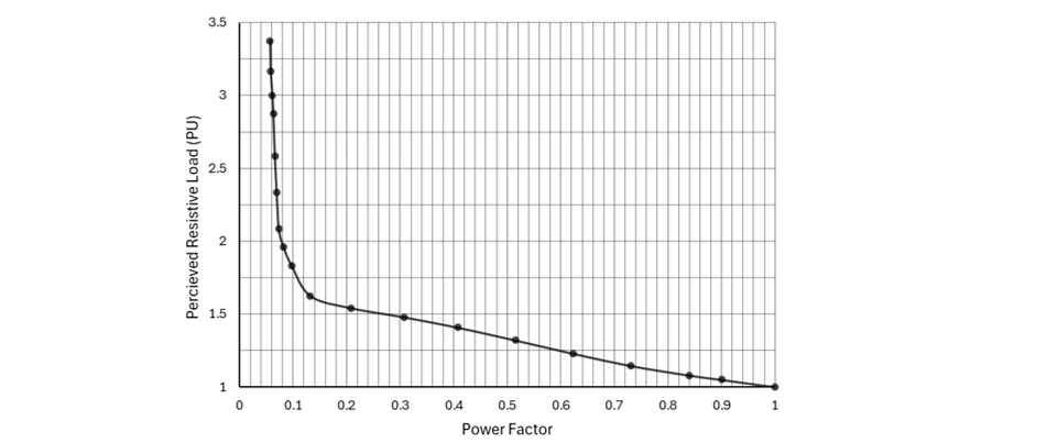
Figure 2 - A 1pu resistive load measured as a function of power factor
Most jurisdictions apply limits to the Overall Error permitted for metering installations for which they are responsible. As the annual energy throughput increases, these limits generally become tighter, requiring a higher class of both instrument transformers and energy meters. Unfortunately, even with Class 0.2 meters and instrument transformers, the OE still becomes excessive as the power factor falls toward zero.

4. Active Energy Metering in Synchronous Condensers
The anomaly outlined above has not generally caused metering difficulties in the past because active power is seldom supplied at extremely low power factors. However, with the resurgence of synchronous condensers and the need to measure their running power, it is now becoming a problem. Some network owners who do not appreciate this have planned a conventional approach to metering these machines, that just will not work. Instead, a more analytical approach must be taken and the energy consumed calculated for each metering interval.
Figure 3 shows a simplified one-line-diagram of a typical synchronous condenser installation. Because these machines operate at medium voltages (typically 11-15kV), a step-up transformer is needed as an interface to the local transmission potential. Three auxiliary supplies are provided; one for the machine field supply, one for the pony motor, (or in some cases an MV static frequency converter), used to run the machine up to synchronous speed prior to startup, and one to provide a supply for all the auxiliary equipment required for the installation.
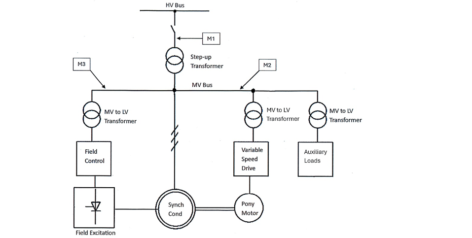
Figure 3 - A simplified one-line-diagram of a synchronous condenser installation
Shown in Figure 3 are three energy meters, M1, M2 & M3, all of which will be used in the calculation of the active energy consumed by the installation during each metering interval. This will initially be calculated in terms of the power loss in kW and then converted into energy (kWh), by multiplying by the metering interval length, expressed in hours.
At this point it is instructive to list the main sources of loss that must be included in the calculation:
- The friction and windage loss that must be supplied by the network to run the machine
(This will also include the losses associated with an external flywheel and the magnetizing losses associated with the step-up transformer.)
- The field power required by the machine
(This is a function of the machine’s reactive power output, as illustrated by the graph in Figure 4, and measured by meter M3, if provided. Alternatively, the field power may be calculated from the average reactive output of the machine; measured by M1.)
- The power required for start-up purposes as well as the auxiliary equipment required for the installation; measured by M2
- The synchronous condenser stator and the step-up transformer copper losses
(These will be calculated from phase current measurements recorded by M1.)
4.1. Machine Friction and Windage Losses (Running Power, P1)
Because the machine spins at synchronous speed and delivers no active power to the bus, its running power is constant. This information is usually supplied by the manufacturer, however it can be measured during commissioning, provided that the machine is neutrally excited to generate no reactive output power, to avoid incurring stator and transformer copper losses. This measurement will be designated P1 and will include the small neutral excitation loss in the field, (shown in Figure 4). P1 should also include the magnetizing losses associated with the step-up transformer.
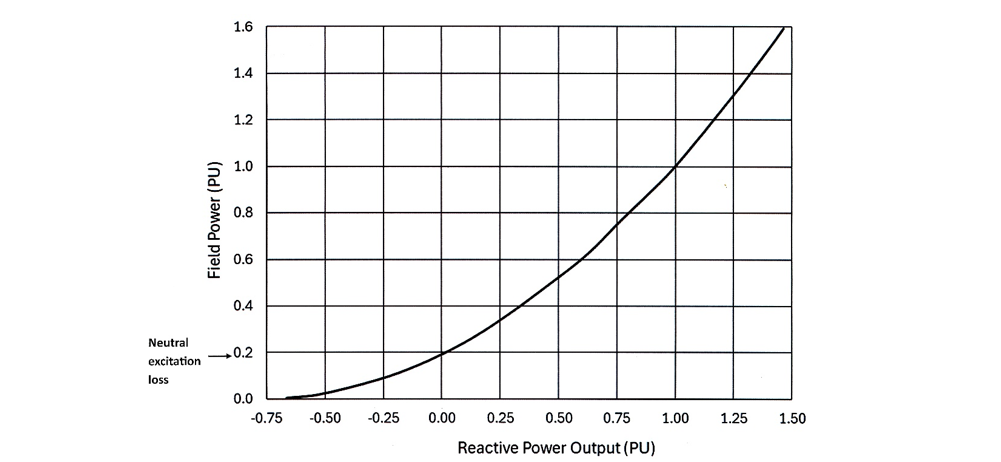
Figure 4 - Typical field power required as a function of the reactive power generated
4.2. Field Power (P2i)
The field power required depends on the reactive power generated by the machine, measured by M1. The relationship between these two quantities will be provided by the machine manufacturer in the form of a graph, similar to that in Figure 4. The field power can either be measured by M3, (if fitted), or it can be calculated as follows:
The reactive energy measured by M1 for the current metering interval, can be converted to the average reactive power by dividing it by the metering interval length, expressed in hours. From this result and the excitation graph provided, the additional field power beyond the neutral excitation component can be found. In either event, the field power for interval i, will be designated P2i.
4.3. Starting & Auxiliary Power (P3i)
The pony motor and auxiliary energy, measured by M2, should be converted to the average power for metering interval i, as described above. This will be designated P3i and will largely represent the associated transformers and auxiliary equipment losses, once the machine has been started. The latter includes cooling and oil pumps, fans, machine heating, HVAC and general power & lighting.
4.4. Synchronous Condenser Stator & Step-up Transformer Losses (P4i)
Both the machine and the step-up transformer copper losses must be calculated. This can be done by programming meter M1 to also record the average phase currents observed throughout metering interval i, which will largely reflect the reactive current in the machine. The copper losses can then be calculated from the machine stator and transformer winding resistances, as provided by their manufacturers.
In principle the copper losses are functions of the tap setting, however, since these will be a small fraction of the overall loss, by using the values corresponding to the principal tap, an acceptable compromise can be made without needing to know the actual tap selected. These losses will be designated P4i.
4.5. Total Energy Calculation
Finally, let the total active power consumed by the complete installation, for the metering interval i, be designated PTi, given by:
Of these elements, P1 will generally be by far the largest. The energy consumed in kWh for interval i, designated Ei, therefore becomes:
Ei = ( PTi x Metering Interval Length ) kWh
The above calculation must be repeated for every metering interval to mimic the data generated by a conventional energy meter.
4.6. Example Calculation
The following example relates to a small 11kV, 40MVAr synchronous condenser, connected to a 110kV bus via a step-up transformer. We consider the case where machine is running and exporting reactive power at its nameplate rating, and will assume that the metering interval is 30 minutes. The step-up transformer’s copper and magnetizing losses as reported by the manufacturer are 120kW, and 30kW respectively. The friction, windage and neutral excitation losses for the machine and its flywheel (P1), reported by the manufacturer is 780kW, plus 30kW magnetizing loss from the step-up transformer, yielding a total of 810kW for P1. Alternatively, this can be measured by M1 under neutral excitation.
Excitation Loss, P2i
From the excitation curve supplied by the manufacturer (not shown), the machine requires 70kW excitation to export 40MVAr to the network, and the neutral excitation required for Q = 0, is 15kW. Therefore, the additional excitation power required for full output is P2i = 55kW.
Starting and Auxiliary Supply Losses, P3i
This energy was measured by M2, and for this metering interval the meter recorded a total of 75kWh. Therefore, the average power supplied becomes:
75kWh/0.5h = 150kW = P3i
Synchronous Condenser and Step-up Transformer Losses, P4i
The machine current as seen at the 110kV bus at full load, is 210A. This can either be calculated from the M1 interval data or obtained from the meter, as described in section 4.4. In this case the machine and transformer winding resistances as referred to the 110kV bus, total 1.27Ω. Therefore, the total copper loss will be:
210² ∗ 1.27Ω ∗ = 168kW
Therefore P4i = 168kW.
The total loss associated with the machine installation is therefore:
PTi = (P1 + P2i + P3i + P4i ) = 810 + 55 + 150 + 168 = 1183kW
This must now be converted to the energy that would have been recorded by a conventional meter, Ei:
Ei = (PTi x Metering Interval Length) = 1183kW ∗ 0.5h = 591.5kWh
In this case the power consumed at full output represents about 3% of the machine’s nameplate rating. Had this been metered with a conventional installation, which under these conditions could easily have an Overall Error of about 150%, then an energy of around 1500kWh would have been recorded instead.
5. Conclusion
Where synchronous condensers are owned by the network operator, the metering of the associated losses may not be considered important, since these may be considered part of the overall network loss. However, when they are owned by a third-party, (for example, the operator of a wind or solar farm), it is, in the opinion of the author, important to ensure that the owner is not overcharged for the energy supplied to operate the machine.
Reference
- G. Vertigan “AC Circuits and Power Systems in Practice” Hoboken, NJ, USA, Wiley, 2017, p. 367 – 372.
Biography
Graeme Vertigan graduated from the University of Tasmania with a degree in Electronic Engineering in 1978. He has worked in heavy industry and has been a consulting engineer since 2012, prior to which he also spent several years teaching at the same university. He has extensive experience in field of energy metering and has run metrology courses for the Australian Energy Market Operator since 2007.