Enhanced Modelling and Parameter Determination of HVDC Cables Using Practice-Oriented Methodology
Authors
T. KARMOKAR - TenneT TSO GmbH, Germany & Delft University of Technology, The Netherlands
M. POPOV - Delft University of Technology, The Netherlands

Summary
HVDC cable systems are vital for long-distance power transmission, especially for offshore wind energy. The point-to-point HVDC transmission links are already in use. For enhanced system reliability, interconnected DC network with fault separation devices like DC circuit breakers are envisaged. This requires the evaluation of the interface between DC cables and circuit breakers for different contingency scenarios. Electromagnetic transient simulations are commonly employed for HVDC network analysis. This paper proposes a practice-based approach to accurately model cable systems, which are crucial for reliable HVDC network analysis. It emphasizes considering real-world implications of cable manufacturing and installation conditions. By enhancing existing knowledge of cable parameter determination, this study proposes practical models using EMT simulations. The aim is to provide engineers with a systematic method to convert DC cable data into EMT-compatible parameters, facilitating representative modelling for thorough HVDC network performance assessment. This is vital for defining specifications of complex HVDC systems, particularly multi-terminal networks.
Keywords
EMT simulations, HVDC cables, Network reliability, Parameter determinationNomenclature
- HV: High Voltage
- HVDC: High Voltage Direct Current
- MT-HVDC: Multi-terminal HVDC
- EMT: Electromagnetic Transient
- VSC: Voltage Source Converter
- DCCB: DC Circuit Breakers
- XLPE: Cross-linked Polyethylene
- HDPE: High Density Polyethylene
1. Introduction
HVDC cable systems are a promising and irreplaceable technology for the reliable transmission of bulk power over long distances, particularly for offshore wind energy, which represents a new horizon for clean energy utilization [1]. These cable systems are crucial in building the energy highways necessary to meet the growing electricity demand. While HVDC cable systems have already been implemented for point-to-point transmission links [2], there is a growing need to increase their availability and optimize operating expenses by reducing system losses and maximizing the use of transmission infrastructure. An interconnected DC network offers a promising solution by optimizing DC-side connections and providing long-term benefits. It, however, requires fault separation devices, such as DCCB to isolate faulty sections and ensure overall network reliability. The DC cables will thereby electrically interact with the DCCBs, and the impact during different contingencies at this interface needs to be evaluated. EMT simulations are typically used to analyse the performance of grid systems under different operational scenarios.
As the development of grid infrastructure progresses, it becomes crucial for us to assess the electrical interface of HVDC cable systems with representative models that accurately depict real-world practices. A practice-based approach to accurately model cable systems is essential for reliable network analysis. This method effectively facilitates the determination of crucial HVDC system specifications and assesses network reliability criteria. A comprehensive engineering approach for cable-based HVDC interconnections must account for transient voltage and current profiles encountered by cable systems during steady-state operation, including contingency scenarios such as faults. This meticulous consideration is crucial to conducting a thorough analysis of operational stresses, significantly influencing an accurate assessment of HVDC network reliability. The accurate EMT modelling of coaxial DC cables comprising a core conductor and metallic screen is crucial. It greatly impacts the characterization of wave propagation properties and subsequently influences the overall response of the cable model in typical VSC-HVDC studies [3].
This paper deals with EMT simulations to develop practical models that accurately determine and represent cable parameters, which can vary from those employed in ideal coaxial transmission systems. In [4], a method is outlined for deriving cable parameters from its geometrical data and material properties, ensuring compatibility with the Cable Constants routine of an EMT program. The objective of this paper is to enhance the existing knowledge regarding the determination of cable parameters for EMT simulations. This is achieved by examining modern cable designs and employing a methodology focused on practical application, which emphasizes consideration of real-world implications of cable manufacturing and installation conditions. By doing so, this paper presents a more robust approach to modelling various cable layers, offering insights into managing the inherent approximations within the EMT simulation environment, where cable layers are typically treated as geometrical cylinders. As a result, this paper offers a thorough approach to interpreting 525 kV cable data for both land and subsea applications and incorporates it into the Cable Constants routine of the EMT program. The aim is to attain a more precise representation of both the material characteristics and construction attributes of the cable.
Finally, the goal is to provide HVDC system engineers with systematic and ready-to-use formulation to convert available DC cable data into parameters, which could then be directly entered into the EMT simulation tool. Indications have been provided on how to circumvent missing data and derive the actual full-size cable for EMT simulations without missing out on cable layer details. With such a practical approach, a representative EMT modelling of DC cables can be achieved which is crucial to thoroughly study the overall HVDC network performance concerning load flow, contingency, control and protection interaction studies. Thus, decisions can be made regarding the definition of system-level specifications for cable-based transmission networks, which is necessary for the increasingly complex HVDC systems envisaged as MT-HVDC networks [5].
2. Methodology
The investigation employs EMT simulation to analyse the transient behaviour of HVDC cables designed for operation at a voltage level of 525 kV. Simulation parameters are determined analytically, incorporating the latest cable specifications anticipated for various transmission expansion projects up to 2 GW, notably in Germany [6]. The methodology focuses on modelling and analysing the response of HVDC cables to occurring transients, which may arise from short-duration disturbances in the HVDC network, such as unscheduled events including switching operations or faults. By applying a case study approach, the investigation focuses on sensitivity analysis of individual cable layers to gain phenomenological insight into influential cable parameters. The characteristic properties of the cable are specified in terms of its geometrical and electrical data and varied within a defined range to study its behaviour when the cable is exposed to transient oscillations. In this process, established techniques, as in [4] for calculating cable parameters for modern HVDC cable designs are refined and discrepancies are highlighted.
The goal is to develop fidelity models for 525 kV HVDC cables, where the influence of cable joints is currently not included in the study. The developed cable models are represented as simplified single DC poles without additional impedances. The idea behind this approach is to examine the cable model and its parameters independently, without external factors that may arise from parameters outside the cable. For the entire study and each sensitivity analysis of cable parameters presented in the underlying sections of this paper, a simplified representation of a single DC pole cable has been implemented as shown in Figure 1. An ideal voltage source, U0,dc, with a defined rate of rise has been used to apply a constant DC voltage on the cable. For maintaining numerical stability and emulating DC conditions, the voltage is applied with a frequency of 1 mHz [7], using a switch, sw to create a time delay of 1 ms to apply the voltage. A single section of a relatively short cable length of 20 km is chosen to generate multiple reflections. The cable screen is continuously grounded with a small resistance of 1 mΩ to maintain perfect grounding conditions for the cable. The far-end of the cable is kept open by terminating it numerically with a large resistance of 1 TΩ. The far-end voltage reflections, Uf,dc are analysed to study the impacts of cable modelling parameters.
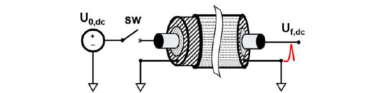
Figure 1 - Schematic of a coaxial cable with an open termination at the far-end to study induced reflection effects in 525 kV HVDC cables
Practical conditions, such as burial depth and soil resistivity are also taken into account. For land cables, a soil resistivity of 100 Ωm is defined while for sea cables, it is considered that the seafloor resistivity is the same as seawater resistivity with a value of 0.3 Ωm [8]. Possible coupling effects between different HVDC cables are not included in the simulation since only one-pole cable is modelled without considering other pole-cable or cables from HVDC networks in the vicinity. The modelled HVDC cable utilizes XLPE insulation with a relative permittivity value of 2.4. Modern XLPE insulation materials for HVDC cables are electrically clean with low conductivity and hence have a low dielectric dissipation factor, tanδ of 10-4, as measured in [9] in the low-frequency range of 1 Hz up to 50°C. This value is appropriate for EMT simulations of 525 kV HVDC network, as higher loss tangents would increase wave attenuation and affect transient response estimation. The dielectric loss, as defined in [10], is a frequency-dependent parameter influenced by both the permittivity, ∈0(ω) and ∈r,ins(ω), and the conductivity, σins of the dielectric medium, specifically the XLPE insulation of the HVDC cable. Since neither of these insulation properties can be defined as frequency-dependent parameters for EMT simulations, and considering the low-loss nature of cable insulation in HVDC applications, the relationship between dielectric loss and these properties can be expressed as shown in (1).
(1)
This correlation directly links the dielectric dissipation factor, tanδ to the conductivity value of the insulation, σins, which in turn exhibits an inverse relationship with the resistance, Rins offered by the insulation to the movement of free charge carriers. For 1 Hz with a tanδ value of 10-4 and a relative permittivity of 2.4, the conductivity of DC-XLPE insulation, σins can be estimated to be about 10-14 S/m.
Furthermore, the conductance, Gins of the insulation governs the leakage current flowing through it, thereby determining the conductivity, σins of the insulation material. The conductance is influenced by both the conductivity of the insulation material and its thickness, as indicated in (2). Based on the estimated insulation conductivity mentioned earlier, the corresponding conductance can be approximated to around 10-13 S/m. This estimation serves as a basis for determining the shunt conductance value of cable models for EMT simulations. However, it is important to note that this value does not consider additional dielectric losses potentially resulting from cable joints where temperature-dependent conductivity in presence of resistive DC field grading may lead to Joule losses. Hence, a conductance value increased tenfold, set at 10-12 S/m, has been used for the presented simulations for both land and subsea cables to account for possible representative dielectric losses along the cable route. This adjustment balances capturing key physical effects in joints with EMT simulation requirements, without risking excessive wave attenuation. Alternatively, if necessary, the dielectric losses due to shunt conductance can be defined based on the loss tangent value of 10-4. In EMT simulations, particularly when modelling extensive cable routes, dielectric loss considerations become crucial. Overestimating the dielectric loss of cables can lead to an exaggerated voltage drop profile throughout the route, whereas underestimating these values can yield less conservative voltage drop outcomes.
(2)
3. EMT Cable Modelling
3.1. Theoretical Basis
Detailed formulation of matrices for the cable impedance, |Z| and admittance, |Y| is necessary to accurately analyse wave propagation characteristics and transients in cable systems [11]. Figure 2 presents an equivalent circuit diagram of a coaxial cable, depicting it as a segment, dx, of a uniform cable with a constant cross-section. The essential elements defining this cable segment include resistance R(dx), inductance L(dx), conductance G(dx), and capacitance C(dx). The currents and voltages are instantaneous values and vary with distance, x, along the entire cable. Accordingly, the impedance and admittance matrices of a cable are defined in (3), (4). The correlation between the matrices |Z| and |Y| is presented in the Appendix.
(3)
(4)
where, N represents the number of parallel conductors. For land cables, N equals 2, consisting of the core conductor and screen, as shown in Figure 3. Particularly for subsea cables, N equals 3, including the core conductor, sheath, and armour, as illustrated in Figure 4.
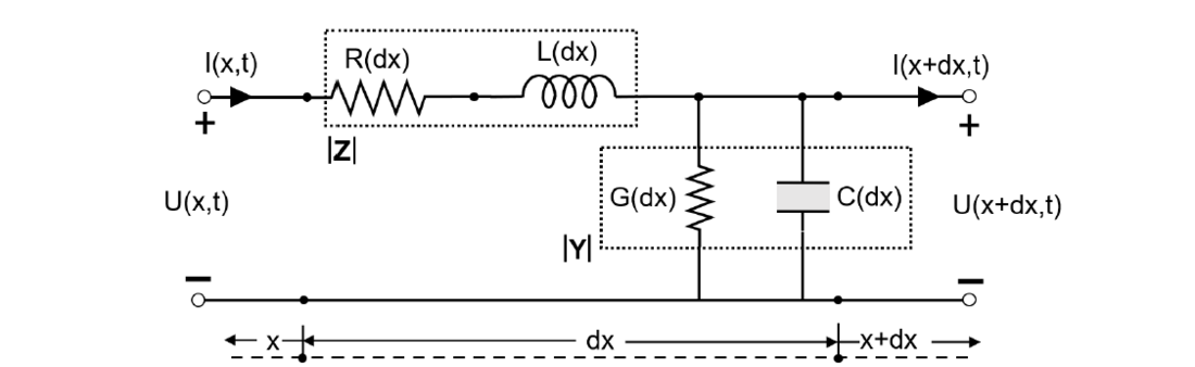
Figure 2 - An equivalent circuit diagram of a coaxial cable with impedance |Z| and admittance |Y|
To accurately model cables in an EMT environment, it is essential to calculate the parameters from cable datasheets to reflect the real cable structure. The mathematical expressions used for EMT cable parameter computations must align with the physical structure and layer definitions of actual cables. Capturing the correct electrical behaviour in EMT requires precise impedance and admittance parameters. The impedance matrix, |Z|, expressed by (3), represents the resistance and inductance of the cable, as shown in (5). Conversely, the admittance matrix, |Y|, in (4), accounts for the cable's ability to conduct electrical current and is the inverse of the impedance matrix, with elements as shown in (6). Both these matrices are symmetrical and relate to current and voltage at both cable ends. Ensuring consistency in these matrices is crucial for accurately modelling the electrical behaviour of the cable in an EMT simulation environment. Both matrices are derived from geometrical and material properties of the cable. The following sections of this paper demonstrate the importance of translating cable parameters from datasheets into the EMT simulation environment while maintaining coherent |Z| and |Y| matrices through parametric variations and sensitivity analysis. The presented analysis in this paper is applicable to all EMT-based software packages.
(5)
(6)
where, Rcab represents the total resistance of the cable, encompassing both the conductor and screen resistances. Lcab denotes the cable inductance. Gins and Cins are the insulation properties, specifying conductance and capacitance, respectively.
3.2. Cable Data for EMT simulations
HVDC cables typically consist of a conductor surrounded by layers of insulation and shielding material. Generally, they include the conductor, triple extruded insulation comprising of inner and outer semi-conductive layers, and the main insulation. The land cable design includes a metallic shielding layer, which is also referred to as a cable screen, and a protective outer sheath. For subsea cables, additional layers of galvanized steel wires are added over the metallic sheath to provide mechanical strength and resistance to water pressure.
Table I provides the essential material and geometrical data of a 525 kV land cable used for practical applications. Figure 3 illustrates the cross-sectional characteristics of the 525 kV land cable with two different screen design variants. Notably, the data in Table I corresponds to the design variant shown in Figure 3 (c).
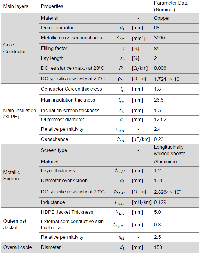
Table 1 - Geometrical and Material Datasheet of a Typical 525 kV HVDC Land Cable
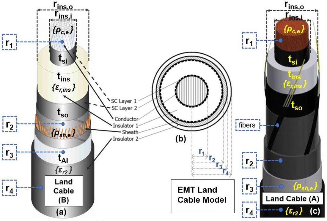
Figure 3 - Comparison of the cross-sectional geometry of a 525 kV land cable in EMT tools to its real-world physical construction: (a) Real-world 525 kV land cable with helically wound copper wires as the cable screen, (b) Cross-section of the land cable model, as seen in EMT software, (c) Real-world 525 kV land cable with a longitudinally welded aluminium sheath as the cable screen
Table II provides the essential material and geometrical data for a 525 kV subsea cable used for practical applications. The cross-sectional features of the 525 kV subsea cable are illustrated in Figure 4.
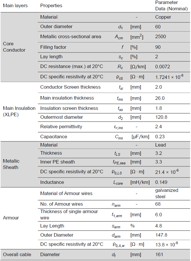
Table 2 - Geometrical and Material Datasheet of a Typical 525 kV HVDC Subsea Cable
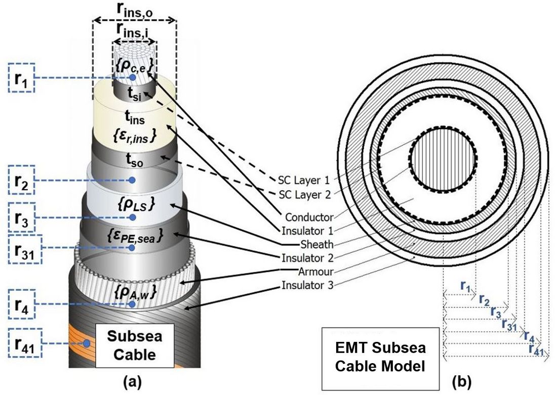
Figure 4 - Comparison of the cross-sectional geometry of a 525 kV subsea cable in EMT tools to its real-world physical construction: (a) Real-world 525 kV subsea cable, (b) Cross section of subsea cable model, as seen in EMT software
4. Computation of HVDC Cable Parameters for EMT Simulations
The arrangement of the cable layers in extruded single-core HVDC cables with modern technology is essentially the same, regardless of the size of the cross-section or the material used in each layer. In this section, the computation of cable parameters is outlined for both land and subsea cables, starting from the innermost layer of the core conductor and moving outwards.
4.1. Core Conductor
The core conductor of a cable, made from either copper or aluminium, transmits the load by carrying the rated current. It consists of intricately wound metallic wires forming a stranded design with a specific lay length, as shown in Figures 3, 4. The outer conductor diameter from the datasheet includes any bedding material within or over the conductor. The key electrical characteristic of the conductor is its DC resistance, determined by its resistivity, crucial for transferring rated power with minimal thermal losses. The relation between the DC resistance and its resistivity is expressed by (7).
(7)
where, ρcm is the maximum DC resistivity of the core conductor that corresponds to its maximum DC resistance, Rc at 20°C.
In EMT-type software, the outer conductor diameter must correspond to its actual DC resistance value. The deviations of the outer diameter or DC resistance of the conductor require adjustments to its DC resistance value, making the originally provided manufacturer’s datasheet values invalid for direct use in EMT simulations. If the conductor DC resistance is unknown or requires validation, (8) can be used to derive it from the specific DC resistivity, ρc0, and the defined lay length, sc, of the conductor, averaged over all strands.
(8)
where, Acm is the metallic cross-sectional area of the core conductor, comprising of the total surface area covered by all strands of the entire metallic core conductor.
From a manufacturing perspective, the stranding process of the core conductor increases its actual resistivity, primarily due to factors like compacting and the presence of semiconductive material within and around the conductor. Such effects could be combined into an overall factor, kf, as seen in (9), which correlates with the lay length, sc, and the filling factor, f, of the particular conductor design to its specific, ρc0, and maximum, ρcm, resistivities.
(9)
In EMT simulations, HVDC cables are often simplified by treating the stranded core conductor as a solid conductor, as shown in Figures 3 (b), 4 (b). This approximation requires the DC resistance value in the EMT software to accurately reflect the real stranded conductor design. Typically, the DC resistance of HVDC cables is specified at 20°C, which shall be used for performing conservative transient analysis. This ensures that cable transients are appropriately considered in EMT simulations even when the cable is relatively under cooling conditions following a particular load profile in HVDC network. Moreover, in EMT studies, skin effect, ys and proximity effect, yp are generally ignored, especially for steady-state computations, as they have minimal impact on transient phenomena due to their short duration. The inclusion of these effects would unnecessarily increase AC conductor resistance, Rc,ac, as seen by (10), leading to additional damping of traveling waves during faults. Therefore, both effects are omitted in calculating the DC resistance of HVDC cable core conductors for both steady-state and transient studies, applicable for HVDC network analysis.
(10)
4.1.1. Results and Discussion
Figure 5 depicts multiple reflections (in p.u.) at the far-end of a 20 km, 525 kV land cable section for varying lay length factors of the same core conductor. The base value of the lay length factor, sc0, is chosen from the datasheet and set at 2%. This value is then varied to 0%, 10%, and 50%. Furthermore, a hypothetical case labelled “inapt,” which ignores the lay length, is included. The results align with (7) and (8), demonstrating a direct relationship between lay length and damping: as the lay length decreases, damping is reduced, and alternatively, as the lay length increases, damping also increases.
At the first peak, the differences are noticeable but minor. However, as the transient progresses, these differences become more pronounced, especially around the 5% band of U0,dc. Increased damping affects the peak value of each successive oscillation and introduces a slight delay in achieving each successive peak. This delay, similar to the damping profile, becomes more evident over time. The 5% band of U0,dc highlights the variation in delay of travelling waves between the “inapt” lay length and the other varying lay length values.
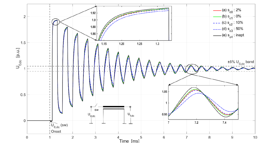
Figure 5 - Comparison of far-end voltage reflections in a 20 km 525 kV land cable with varying lay length factors of the core conductor
4.2. Main Insulation
The primary insulation of an HVDC cable consists of three distinct layers: the conductor screen, also referred to as the inner semiconductive layer; the main insulation, typically made of extruded insulation, and the insulation screen, also known as the outer semiconductive layer. For this investigation, XLPE has been chosen as the primary insulation material. The inner and outer semiconductive layers serve as means to equalize the electric field stress at the outer surface of the core conductor and the inner surface of the metallic screen, respectively. Because both the conductor screen and insulation screen possess semiconductive properties, they exhibit a relatively higher resistivity compared to the core conductor and the metallic screen of the cable. Consequently, no current flow is anticipated within these semiconductive layers. Therefore, for EMT simulations, both of these semiconductive layers are considered integral components of the primary insulation, as seen in (11). These layers can be used to calculate the outermost diameter over the insulation screen or geometrical values can be obtained from the manufacturing datasheet. In EMT-based simulations, the inclusion of such additional semiconductive layers within the primary cable insulation can affect the actual cable capacitance. It is essential to verify whether the EMT cable models can internally account for these adjustments, as implemented in the presented results. If this is not the case the permittivity of the main insulation should be adjusted accordingly to ensure the actual cable capacitance, as shown in [4].
(11)
At times, an offset in the calculated value using (11) may be observed, particularly when additional layers of semiconductive tapes are helically wound over the insulation screen to provide longitudinal water-blocking properties to the cable. These tapes must also be considered as a part of the primary insulation during EMT simulations due to their semiconductive properties. Equation (11) provides a slightly lower value for d2 as compared to the value provided in the datasheet of Table I. This difference is attributed to the presence of semiconductive water-blocking tapes over the insulation screen, which is directly under the metallic screen of the cable.
The capacitance of the main cable insulation is determined using equations (12) or (13), which simplify the computation based on the actual thickness of the main insulation. These equations account for the inner semiconductive layer as part of the core conductor, as their potentials become equal. Additionally, the relative permittivity of the main cable insulation, ϵr,ins, is treated as a constant real number, disregarding relaxation phenomena in the primary insulation during EMT simulations.
(12)
(13)
where, rins,i and rins,o are the inner and outer radii of the main cable insulation, respectively, which can be calculated by (14) and (15).
(14)
(15)
4.2.1. Results and Discussion
The impact of insulation thickness, tin variations, along with the thickness variations of the inner and outer semiconductive layers, s, is investigated for two cross-sectional conditions of the cable:
- Gvar: The overall cross-section of the cable varies depending on the thicknesses of the inner and outer semiconductive layers. In this scenario, all layer thicknesses, including the primary insulation, depicted in Figure 6 as tin,k, remain unchanged.
- Gk: The overall cable cross-section remains constant, regardless of the presence of the inner and outer semiconductive layers. Here, all cable layers except the primary insulation thickness remain unchanged. The thickness of the primary insulation, depicted in Figure 7 as tin,x, is adjusted according to the presence or absence of the inner and outer semiconductive layers to maintain a consistent cable cross-section.
For both conditions, when the inner and outer semiconductive layers are varied, either doubled, s2x, or removed entirely, s0, both semiconductive layers are adjusted simultaneously. Figure 6 depicts multiple reflections (in p.u.) at the far-end of a 20 km, 525 kV land cable section under the “Gvar” condition. The obtained results are in agreement with the discussions in [12], which attribute that the presence of semiconductive layers leads to a decrease in propagation speed. Similar observations are made for the “Gk” condition, as seen in Figure 7.
In the “Gvar” condition (see Figure 6), with a fixed insulation thickness, adding semiconductive screens increases the inductance of the core-sheath loop without altering the capacitance, thus reducing propagation velocity and increasing surge impedance. In contrast, the “Gk” condition (see Figure 7) adjusts insulation thickness to maintain a consistent cable cross-section, leading to a negligible change in inductance but an increase in capacitance due to reduced insulation thickness to accommodate semiconductive layers. This results in a greater reduction in propagation velocity in the “Gk” condition compared to the “Gvar” condition, as shown by the blue curves in Figures 6, 7. Additionally, when the insulation thickness is increased to maintain an unchanged overall cable cross-section in the absence of semiconductive layers, the resulting decrease in capacitance leads to an increased propagation velocity, as indicated by the green curves in Figures 6, 7. To replicate the attenuation effects of semiconductive layers in EMT simulations, it is essential to maintain a coherent cable cross-section for varying layer thicknesses in the insulation system. This consistency ensures that the electrical characteristics, such as inductance and resistance, remain uniform throughout simulations, thereby facilitating accurate modelling of the impact of semiconductive layers on attenuation. Material-level effects introduced by these layers, which cannot be directly simulated in EMT, can only be effectively captured when the cross-section is held constant. By ensuring a consistent cross-section, the influence of semiconductive layers can be isolated from other variables that may introduce discrepancies in the results. While both Figures 6 and 7 illustrate the anticipated propagation delay effects due to the semiconductive layers, it is in Figure 7 that a more realistic representation of the layer’s contributions to the damping of traveling waves, primarily through their role in introducing additional resistive and dielectric losses, is achieved. This detailed analysis enhances the discussions in [12] by providing a comprehensive overview of the influence of semiconductive layers on the transient profile and outlining their inclusion into EMT simulations for varying lengths.
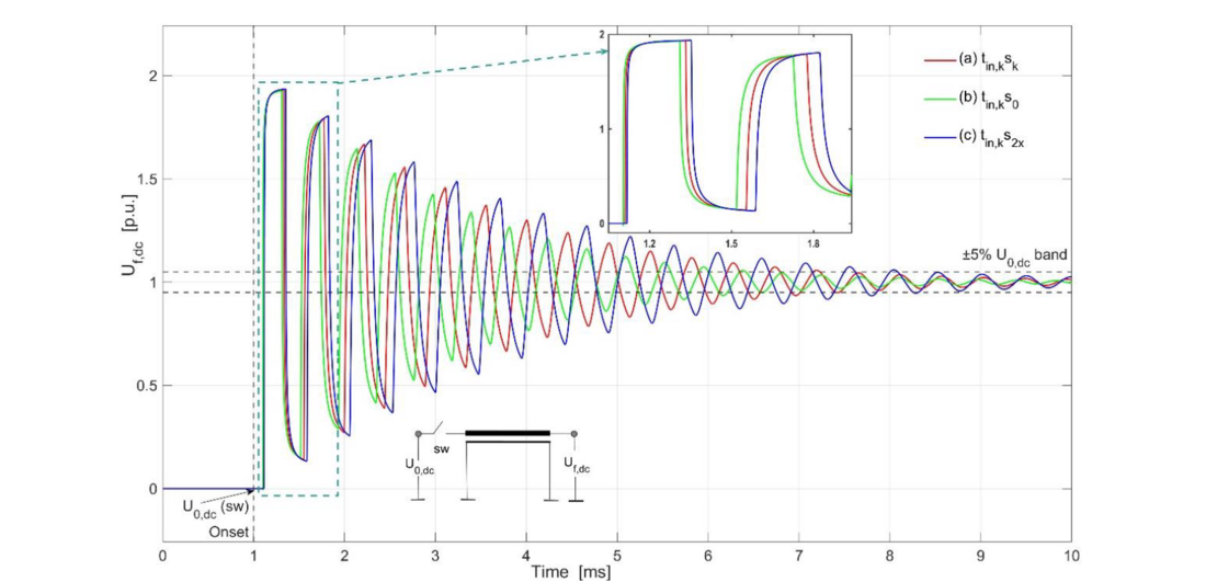
Figure 6 - “Gvar” condition: Comparison of far-end voltage reflections in a 20 km 525 kV land cable with constant insulation thickness and varying thickness of semiconductive layers for incoherent cable cross section
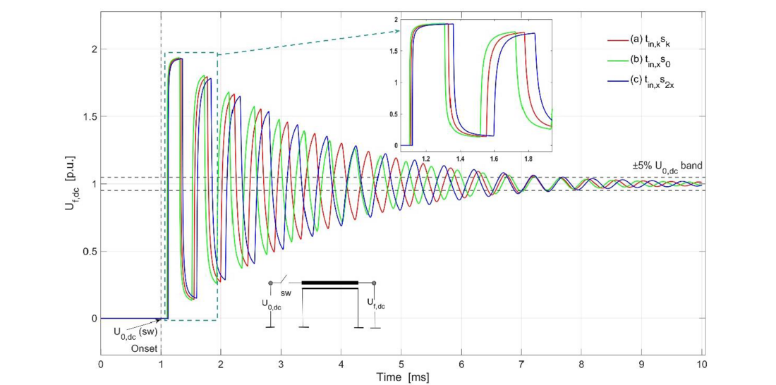
Figure 7 - “Gk” condition: Comparison of far-end voltage reflections in a 20 km 525 kV land cable with varying insulation thickness and varying semiconductive layer thicknesses for coherent cable cross section
In addition to the time domain results, as seen in Figures 6, 7, a frequency scan of the conductor-to-earth impedance is presented in Figure 8, depicting both conditions: “Gvar”, see Figure 8 (a) and “Gk”, see Figure 8 (b). The influence of semiconductive layers is evident from the resonance frequency shifting to a relatively lower value for both conditions (blue curves in Figure 8). Figure 8 (a) illustrates the impact of increased inductance alone, as capacitance remains constant due to unchanged insulation thickness and incoherent cable cross section. However, Figure 8 (b) demonstrates majorly the influence of capacitance for a coherent cable cross section. In addition to the resonance frequency shifting to a relatively lower value, lower impedance is also achieved demonstrating the attenuation effects of semiconductive layers. In contrast, for the “Gvar” condition the attenuation effects due to semiconductive layers is not reflected.
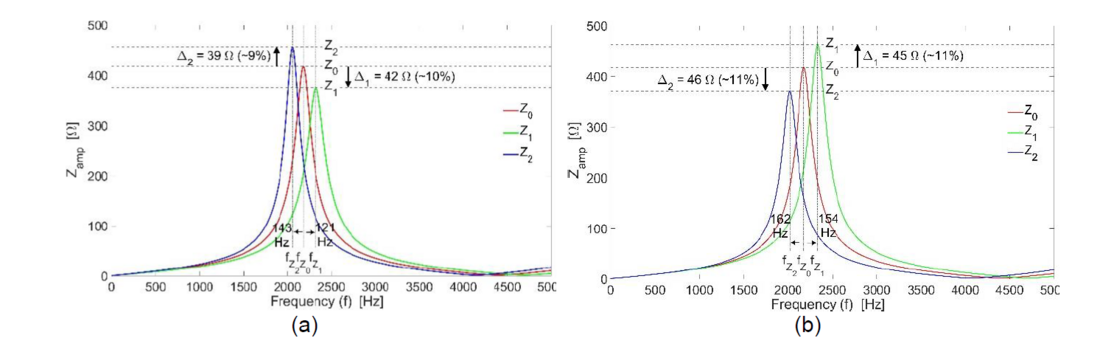
Figure 8 - Impedance profiles as a function of frequency for cable cross-sections, influenced by insulation and semiconductive layer thickness: (a) “Gvar” condition, (b) “Gk” condition. Z0 represents the base case for the actual cable geometry, while Z1 and Z2 depict variations in cable cross sections, with Z1 excluding semiconductive layers and Z2 incorporating twice the semiconductive layer thickness in both the “Gvar” and “Gk” conditions.
4.3. Metallic Screen
The metallic screen of the cable serves as the outermost conductor, ensuring periodic grounding of the cable along its entire length to establish a reference for the operational voltage of the cable. It is not meant to carry the load current, but the fault current and asymmetrical current during system unbalance in service. There are several types of metallic screens for HVDC cables with the most common types of onshore applications being either the copper wire screen together with an aluminium metallic moisture barrier or an aluminium tape sheath. For subsea cables, a typical choice is the lead sheath mainly because of its high resistance to corrosion when the cables are exposed to the moist environment of subsea conditions.
4.3.1. Metallic Screen of Land Cables with Aluminium Sheath Only
If the metallic screen consists of an aluminium sheath, it is applied longitudinally to encircle the cable core. Since the aluminium sheath is in the form of a foil, it cannot be applied by winding it helically around the cable core. Instead, it is either longitudinally welded or adhered over the insulation screen and a semiconductive longitudinal water barrier. This arrangement serves multiple purposes, including ensuring radial water tightness, providing mechanical protection, and serving as a pathway for fault and asymmetrical currents during service. The area; AAl covered by the aluminium sheath can be computed by (16). Its DC resistance; R0,Al and the corresponding DC resistivity; ρ0,Al, both at 20°C are computed by (17) and (18) respectively.
(16)
(17)
(18)
4.3.1.1. Results and Discussion
The far-end voltage reflections for a 20 km, 525 kV land cable equipped with an aluminium sheath as the metallic screen are illustrated in Figure 9. The comparison evaluates the cable considering the actual resistivity, ρAl,s0,real of the screen, as outlined by (18), versus a scenario where the same cable is modelled by ignoring the geometrical properties of the metallic sheath. Instead, it solely utilizes the DC-specific resistivity of the aluminium material for the cable screen, denoted as ρAl,s1,inapt in Figure 9. The results demonstrate that neglecting geometrical details and relying solely on material properties to calculate the resistance of the metallic screen leads to a substantial decrease in the attenuation of the transient inside the cable.
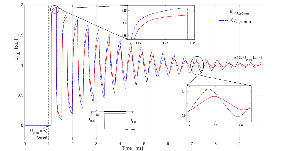
Figure 9 - Comparison of far-end voltage reflections in a 20 km 525 kV land cable with an aluminium sheath as the metallic cable screen, emphasizing the impact of its resistance on cable transients
4.3.2. Metallic Screen of Land Cables with Copper Wires
The wire screen, as seen in Figure 3 (a), is composed of circular copper wires, having the diameter of each wire as ∅1,Cu,w in mm, wound helically around the cable core with a particular lay length, ss. For providing longitudinal water tightness, a layer of semiconductive water-blocking tapes with a thickness of tWL in mm are wound radially over the copper screen wires. Thereafter, a radial water barrier layer made of aluminium foil with a thickness of tAL in mm, is also present. Thus, the diameter d3,Cu in mm , over the copper wire screen in an HVDC cable can be calculated by (19).
(19)
The DC resistance, R0,Cu,w in Ω/km, of the copper wires at 20°C having a specific DC resistivity, ρ0,Cu,w in Ωm is given by (20).
(20)
where, the cross-sectional area, ACu,w in mm² of n number of copper wires forming the metallic screen of cable is given by (21)
(21)
The overall DC resistance and resistivity of the metallic cable screen is an equivalent value, provided by R0,sh,e as seen in (22) and ρ0,sh,e as seen in (23), respectively, due to the equipotential connection between the copper wires and the aluminium laminate at grounding locations along the cable route length.
(22)
(23)
Thus, the effective cable screen diameter d3,e, in mm , over the aluminium sheath with the copper wires underneath and the layer of semiconductive water-blocking tapes in between can be calculated by (24). This must then be used as the geometric parameter for EMT land cable models with copper wire screen design.
(24)
4.3.2.1. Results and Discussion
Figure 10 illustrates the far-end voltage reflections for a 20 km, 525 kV land cable equipped with a metallic screen made of copper wires. The comparison evaluates the cable screen with its actual resistivity, ρCu,s0,real, determined using (23), against alternative copper wire screen design variants to demonstrate their effects on the attenuation profile of cable transients. These design variations include a configuration with a zero lay length, ρCu,s1,zero, and a case where the screen is modelled as a copper sheath, ρCu,s2,sheath instead of individual wires. Additionally, scenarios where geometrical details, typically accounted for in (23), are disregarded, and only the copper material properties are used to calculate the screen resistance, ρCu,s3,inapt are explored. These latter configurations are theoretical and serve to highlight the importance of accurate cable screen modelling. Finally, results for the same cable equipped with an aluminium sheath, ρAl,s4,real, as the metallic screen are included, showcasing the differences in attenuation characteristics between copper and aluminium sheaths.
The results indicate that reducing the lay length of copper wires from their actual value, ρCu,s0,real to zero, ρCu,s1,zero notably decreases the attenuation profile. Furthermore, the modelling of the metallic screen resistance as a continuous sheath, ρCu,s2,sheath significantly reduces the attenuation, nearing the lowest attenuation (i.e. highest transient peaks) achieved for the screen resistivity of ρCu,s3,inapt. Interestingly, the aluminium sheath, ρAl,s4,real as the metallic screen, as determined using (18), results in significantly lower attenuation compared to a metallic screen made of copper wires for the same cable core diameter. This is attributed to the lower resistance offered by a continuous aluminium sheath compared to the selected number of copper wires. An equivalent metallic screen resistance with copper wires to that of an aluminium sheath can be achieved by adjusting the lay length of the copper wires, as expressed by (20), and modifying the number and diameter of the copper wires, by applying (21). The results presented in Figure 10 are in agreement with the discussions in [13], which indicate that cable damping characteristics are highly sensitive to the pitch angle (referred to as lay length in this paper) of the screen wires used as the metallic screen. As the pitch angle of the screen wires increases, the surface transfer impedance also increases, affecting the damping characteristics [14]. It is noteworthy that at high frequencies, the skin effect could significantly influence the effective resistance of the cable screen. While cables with aluminium sheaths and concentric copper wires may have the same DC resistance, copper wires generally exhibit lower AC resistance due to more even current distribution, thereby reducing the skin effect. The higher conductivity of copper results in a smaller skin depth, nevertheless allowing greater current flow and minimizing losses during high-frequency events. However, since these high-frequency phenomena are short-lived, typically lasting tens to hundreds of milliseconds, their effects are minimal and are not examined in detail in this study.
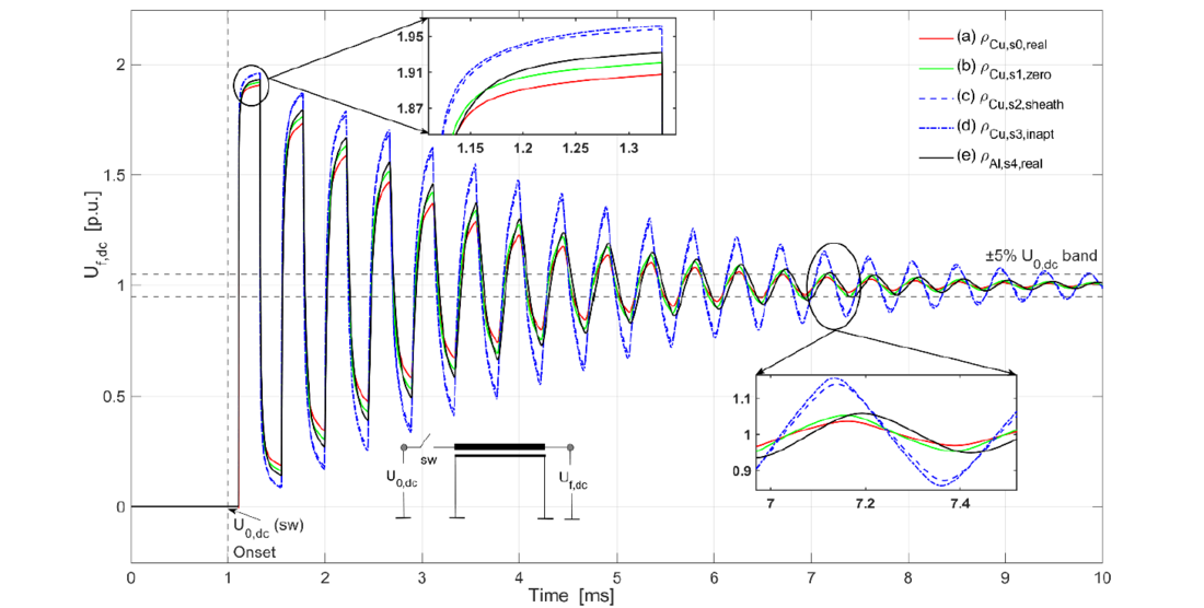
Figure 10 - Comparison of far-end voltage reflections in a 20 km 525 kV land cable with copper wires as the metallic cable screen, emphasizing the impact of its resistance on cable transients
4.3.3. Metallic Screen of Subsea Cables with Lead Alloy Sheath
The diameter over the lead sheath; dLS in a subsea HVDC cable is calculated by (25)
(25)
The DC resistance offered by the lead sheath can be calculated using (26)
(26)
The parametric variations of lead sheath thickness have been excluded from this paper. Analogous to the conducted analysis as seen in Figures 9, 10, increasing its resistance by reducing the thickness of the lead sheath, which is the designated metallic sheath for subsea cables, increased attenuation of cable transients are achieved. This finding aligns with the discussions in [12].
4.4. Cable Oversheath
In general, the metallic screen of HVDC cables is typically grounded at regular intervals along its entire route length. As a result, its potential remains low, if not at earth's potential, compared to the core conductor, even during transient conditions. Consequently, the simulated transients on the core conductors are not significantly influenced by the properties of the insulating materials external to the metallic screen.
4.4.1. HDPE Outermost Jacket of Land Cables
The outermost HDPE jacket of land cables may not have a significant impact on the transient performance of these cables. Nevertheless, to ensure the overall integrity of the land cable model, it is important to maintain the same diameter for the outer sheath as that of a real cable. An HDPE outer sheath is extruded over the aluminium foil, providing sufficient mechanical protection during both installation and operation. Additionally, the outer sheath typically includes a thin semiconductive layer, which is applied simultaneously with the underlying HDPE sheath. This semiconductive layer serves the purpose of performing sheath integrity tests before the cable leaves the factory and after it has been installed in the field. The diameter over the land cable outermost jacket, d4 can be calculated by (27) depending on the underlying screen design of the land cable. Thus, the underlying diameter must either be chosen as d3 for the screen with only aluminium sheath or d3,e with screen design with both copper wires and aluminium sheath.
(27)
where, d3,s can either be chosen as d3 or d3,e depending on the screen design of the HVDC land cable.
4.4.2. HDPE Inner Sheath of Subsea Cables
In subsea cables, there is an inner sheath made of HDPE that is extruded over the lead sheath during the same manufacturing process. This HDPE sheath serves multiple protective purposes for the underlying lead sheath. It provides crucial safeguarding against mechanical damage and fatigue by offering mechanical reinforcement to the lead sheath. Additionally, it acts as a barrier to protect the lead sheath from corrosion by minimizing its exposure to oxygen. The diameter over the lead sheath, dLS in a subsea HVDC cable, whose permittivity is specified in Table II, is given by (28):
(28)
4.5. Armour in Subsea Cables
Subsea cables often incorporate armour wires designed to withstand significant mechanical stresses encountered in their underwater deployment. These stresses are particularly pronounced in the depths of the subsea environment where the cables are laid. Furthermore, during manufacturing and the process of loading onto cable-laying vessels, these subsea cables are subjected to bending and torsional forces that they must endure to prevent any damage. Typically, the tensile armour consists of a single layer comprising narm number of round galvanized steel wires, each having a thickness, t1,arm. These steel wires are applied helically around the inner polyethylene layer of the subsea cable with a particular lay length sarm. The aim is to maintain minimal gaps between each armour wire, and in this way, to ensure effective cable protection. Additionally, a rubber-coated tape is commonly utilized as a bedding layer beneath the armour, and the armour wires are impregnated with bitumen to provide effective protection against corrosion.
The diameter, darm over the armour layer in a HVDC subsea cable can be calculated by (29):
(29)
The DC resistance, R0,A,w of the armour wires at 20°C having a specific DC resistivity, ρ0,A,w is given by (30):
(30)
where, the total cross sectional area, AA,w of narm number of armour wires can be calculated by (31):
(31)
Accordingly, the DC resistivity of the armour layer is given by ρ0,A,w as per (32):
(32)
4.5.1. Impact of Ferromagnetic Armour on Modelling of Subsea Cable Screen
The steel wires employed to create the armour layer in subsea cables undergo a galvanization process. This process involves the application of a protective zinc coating onto the steel wires to safeguard them against corrosion. Due to the steel galvanization process, the magnetic properties of the armour material cannot only be determined by its composition but also by the cumulative effects of thermal treatment and mechanical stresses during manufacturing, as well as handling during subsequent processes. Moreover, the magnetic properties of galvanized steel depend mostly on the thickness of the film and the deposition mode, such as hot dip [15]. The exact description of these properties is challenging since to obtain reliable values, it is necessary to measure the internal impedances of the armour as a function of frequency and the pre-magnetization current at the fundamental frequency [16]. For cable applications, the permeability of the armour wires is dependent on the expected magnetic flux density within the wires. The magnetic field is determined by the inductance, which is based on the linkage of the flux to the current generating the flux. As it is discussed in [16], the longitudinal permeability (μL) value can be approximated as 400. It is a complex number and is determined by the eddy currents and hysteresis losses, both of which are negligible in DC cables due to the absence of rate of change of magnetic field. For DC cables, the relevant permeability value for the armour is the transversal permeability, μT. This is crucial for EMT studies where the focus lies on analysing transients using traveling wave theory, impacted by the armour’s resistance, not reluctance, thus creating attenuation effects in sea cables. For EMT simulations, the relative permeability, μr, of the armour layer in subsea HVDC cables, influenced by factors such as wire diameter, lay length, and discontinuities between armour wires, can be approximated to a μT value of 10, as indicated in [16]. This is a reasonable assumption for EMT simulations under the consideration that each armour wire is fully in contact with its adjacent wires, thus creating a negligible air gap between each armour wires. Additionally, high-frequency transient events in HVDC networks are short-lived, typically lasting tens to hundreds of milliseconds. Therefore, estimating μr as 10 prevents overestimation, which would otherwise exaggerate attenuation effects and compromise simulation accuracy. In the case of air gaps, the armour permeability can be reduced and maintained close to unity.
The EMT HVDC cable models for ferromagnetic armour are highly simplified. In the absence of measured data, the DC resistance of the armour layer can be calculated based on the number of galvanized steel wires and their lay length. If the PE sheath is insulated, the armour resistance is considered in parallel with the DC resistance of the lead sheath to determine the equivalent DC sheath resistance of the subsea cable. This is due to periodic equipotential connections between the lead sheath and armour wires along the subsea cable route. If the PE sheath is semiconductive, no additional equipotential points are needed, as sheath bonding occurs through the semiconductive PE sheath, creating a high impedance path to the earth for sheath currents. This contrasts with the insulating PE sheath, which is regularly shorted with armour wires, potentially lowering the impedance to earth for sheath currents. For analysing transients in subsea cables, the coaxial travelling waves between the core conductor and metallic sheath must be simulated. For this purpose, the lead sheath, PE sheath, and armour can be considered as equipotential layers. Accordingly, in the EMT model, these layers can be simulated in contact with water, i.e., perfectly and continuously earthed along the entire subsea route. For the presented analysis, an insulating PE sheath has been implemented. Nevertheless, when investigating the occurrence of transient voltages between the sheath and armour, especially when there is no equipotential bonding between the two layers, it is essential to consider the presence of the semiconductive PE sheath [17]. Additionally, to accurately assess sheath currents in subsea cables, consider the distinct material properties of the PE sheath and the associated grounding technique. These factors determine the effective path of the sheath currents [18].
4.5.1.1. Results and Discussion
The estimation of armour permeability is important for the EMT modelling of subsea cables. Figure 11 presents outcome of techniques in modelling the subsea cables that could essentially be implemented for estimating the armour permeability. Two of the techniques implement different methods to model the sheath – one is by aggregating the lead sheath with the armour and the other by recalculating the thickness of the lead sheath based on the manufacturer provided coaxial inductance value as per (33). Lcoax is mainly determined by the geometry of the core conductor (its outer diameter, d1) and cable screen (its inner diameter, d2 determined as per (11)) for a particular cable design. Both these sheath modelling approaches have been implemented in this study for an insulating PE sheath.
(33)
For the aggregated sheath model of the HVDC subsea cable, an effective sheath resistance is computed based on the equipotential connections between the lead sheath and armour. Essentially, this resistance is equivalent to the parallel DC resistance of the lead sheath and armour, which can be computed based on (26), and (30). The modelling approach combines the sheath and armour into a single layer [19], however by effectively treating the resistance of the aggregated single sheath layer as parallel resistance because the lead sheath is expected to carry asymmetrical currents, and the equipotential bonding with armour provides the earth reference. The outcome is labelled in Figure 11 as Shagr.
In the equivalent sheath model of an HVDC subsea cable, the inner diameter of the lead sheath is adjusted to lie between its actual geometric position and the armour layer, based on the derived inner lead sheath diameter from the coaxial inductance value provided by the manufacturer, as indicated by (33), rather than the diameter from the datasheet. As a result, the lead sheath may become thinner, with its inner diameter moving closer to its outer diameter, for an outer diameter value of the lead sheath maintained as per the datasheet. This adjustment increases the geometric ratio, , signifying a larger area for magnetic flux. This maybe because the lead sheath thickness was likely considered in d2 for Lcoax computation, as per (33), by the manufacturer, although the geometric wall thickness of lead sheath, tLS, remained unchanged. Despite these adjustments, the outer diameter of the lead sheath, dLS as determined by (25) remains unchanged i.e., as per the datasheet.
The resulting decrease in the derived thickness of the lead sheath leads to higher resistivity, affecting the attenuation characteristics of the coaxial transient waveform. In this model, the lead sheath and armour are treated as separate layers with a reduced lead sheath thickness. To maintain the overall cable diameter, the insulation thickness is increased to compensate for the reduction in the derived lead sheath thickness, and the permittivity of the insulation is increased accordingly to maintain a constant cable capacitance. This approach, denoted as Sheq in Figure 11, introduces a time delay due to the increased permittivity, although an unchanged overall cable diameter is maintained.
Varying the permeability of the armour wires for DC applications shows that a permeability of 10, as seen for Shg,μA10 in Figure 11, aligns with the amplitude given by Sheq and is consistent with the recommendations in [16], which suggest an armour permeability of 10. In contrast, using an armour permeability of 1, while keeping the manufacturer’s data unchanged, results in slightly less damped transient behaviour. Therefore, the recommended approach for modelling subsea HVDC cables is to retain the geometrical data provided by the manufacturer while applying an armour permeability of 10.
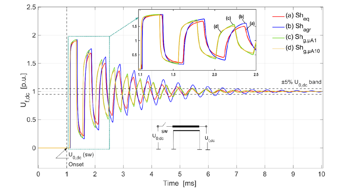
Figure 11 - Comparison of far-end voltage reflections in a 20 km 525 kV subsea cable with different approaches to model the metallic lead sheath of the cable including the armour wires, emphasizing the impact of its sheath resistance on cable transients
5. Conclusion
This paper addresses the lack of realistic data on 525 kV HVDC cables that can be used for network analysis. Apart from presenting data for both land and subsea cables, the paper also guides how to compute cable parameters for EMT simulations by taking into account the practicalities. This information can be used to create realistic cable models for EMT simulations, leading to more accurate and reliable results, which ultimately facilitate dependable decision-making regarding cable stresses.
Thorough models for HVDC cables have been developed which are based on a practice-based approach so that realistic cable interfaces in HVDC networks could be defined, especially with DC circuit breakers. The paper describes such a practice-based cable modelling approach in EMT simulation environment to assess the electrical interface of HVDC cable systems with representative models that accurately depict real-world practices. The presented approach captures realistic cable characteristics in EMT modelling so that representative stress can be studied on cables. The emphasis remains not to simply transfer the cable datasheet values into the EMT simulation environment but to make an attempt to account for the inherent approximations in the simulation tool for adapting the approach to calculate cable parameters.
This paper details such an approach. Moreover, factors related to cable manufacturing have also been discussed. This shall enable a thorough computation of cable parameters in situations when not every parameter can be known from the available datasheet. An approach has been presented to estimate such factors and thereby the outcome of cable transient simulations can be discussed based on the assumptions made. This provides a framework to understand the range within the achieved simulation outcome, thus enabling the definition of tolerance on such simulation results, especially considering the contribution of the HVDC cables.
6. Appendix
Here a mathematical correlation between the impedance |Zcab| and admittance |Ycab| of coaxial cables are derived using the theory of ABCD Transmission Matrix (|ABCD|). The goal is to show how these two parameters: |Zcab| and |Ycab|, are interrelated and influencing each other, which is usually not consciously considered while modelling cables in EMT simulation.
The first step is to transform |Zcab| to |ABCD|. The |Zcab| is known for the cable systems as presented below whereas the |ABCD| is to be determined. The theory of ABCD Matrix reduces an n-port network to a 2 x 2 network and implements a cascade of 2 x 2 systems. Therefore, the transmission line, in this case, coaxial cable, has been expressed as a two-port network comprising of a two-conductor system including the core conductor and cable screen. For this analysis, the approach is considered applicable to both land cable and subsea cable systems, which consist of a sheath as well as metallic armour. The reason why the approach is also applicable to subsea cable systems is that the subsea cable system is typically considered continuously earthed through the seawater.
(34)
The negative sign of screen current is due to the convention of its direction being opposite to that of the current in the core conductor.
(35)
Solving [Zcab] for ABCD parameters:
(36)
(37)
From ABCD Matrix
(38)
(39)
Equations (36), (37) are used to derive ABCD parameters in (38), (39). The derivation is performed for different in-service scenarios concerning the electrical characteristics and grounding conditions of the cable systems.
Determining “A” parameter
For a symmetrical system or a cable system with broken screen wires no current in the cable screen can be assumed. This means Is = 0. Accordingly, from (38) the underlying relation for a voltage ratio, as seen in (40), is achieved.
(40)
Substituting for Uc and Us in (40) from (36) and (37) respectively with Is = 0 we get the voltage ratio defining parameter A as seen in (41):
(41)
Determining “B” parameter
For a perfectly grounded cable system with its screen solidly bolted to earth, the short circuit resistance can be calculated by considering Us = 0.
For Us = 0, (37) can be re-written as follows:
Substituting this relation in the above “B” relation:
Determining “C” parameter
Open circuit conductance with Is = 0, the following ratio can be expressed:
Determining “D” parameter
Current ratio
(42)
Determining the admittance |Ycab| parameters of a coaxial cable in terms of its impedance |Zcab| parameters, thereby establishing the correlation between the |Ycab| and |Zcab| parameters:
Accordingly, the [Ycab] can be defined as follows:
(43)
(44)
(45)
The |ABCD| formulation as seen in (38), (39) remains unchanged.
Simplify (38) and solve for Is.
(46)
Comparing Is in (46) with that in (45) we get (47), (48)
(47)
(48)
Now substitute (46) into (39) and solve for Ic to get (49):
(49)
Equations (46), and (49) can be respectively correlated to (45), and (44) to determine the elements of the [Ycab] matrix as seen in (43):
(50)
(51)
(52)
(53)
(54)
References
- Europacable, “An Introduction to High Voltage Direct Current (HVDC) Subsea Cables Systems”, Brussels, 16 July 2012, EU Transparency Register ID 4543103789-92.
- ENTSO-E, “HVDC Links in System Operations”, Brussels, 2 December 2019, Technical paper.
- A. Beddard and M. Barnes, "HVDC cable modelling for VSC-HVDC applications," 2014 IEEE PES General Meeting | Conference & Exposition, National Harbor, MD, USA, 2014, pp. 1-5, https://doi.org/10.1109/PESGM.2014.6939059.
- B. Gustavsen, "Panel session on data for modeling system transients insulated cables," 2001 IEEE Power Engineering Society Winter Meeting. Conference Proceedings (Cat. No.01CH37194), Columbus, OH, USA, 2001, pp. 718-723 vol.2, https://doi.org/10.1109/PESW.2001.916943.
- A. Shetgaonkar, T. Karmokar, M. Popov and A. Lekić, “Enhanced Real-Time Multi-Terminal HVDC Power System Benchmark Models with Performance Evaluation Strategies”, CIGRE Science & Engineering (CSE) Journal, CSE N°32, February 2024.
- Website of the Federal Electricity Network Agency of Germany “Bundesnetzagentur”: News release dated 01. March 2024.
- H.M.J. De Silva, Z Liu, “An Enhanced Method to Achieve Exact DC Values for Frequency-dependent Transmission lines”, Electric Power Systems Research, Volume 223, 2023, 109649, ISSN 0378-7796, https://doi.org/10.1016/j.epsr.2023.109649.
- S. Constable, “Conductivity, Ocean Floor Measurements” In: Gubbins, D., Herrero-Bervera, E. (eds) Encyclopedia of Geomagnetism and Paleomagnetism, 2007, Springer, Dordrecht, https://doi.org/10.1007/978-1-4020-4423-6_30.
- T. Liu, J. Fothergill, S. Dodd, U. Nilsson, “Dielectric spectroscopy measurements on very low loss crosslinked polyethylene power cables” 2009, Journal of Physics: Conference Series 183 012002, https://doi.org/10.1088/1742-6596/183/1/012002.
- W. S. Zaengl, “Dielectric spectroscopy in time and frequency domain for HV power equipment. I. Theoretical considerations," Sept.-Oct. 2003, IEEE Electrical Insulation Magazine, vol. 19, no. 5, pp. 5-19, https://doi.org/10.1109/MEI.2003.1238713.
- A. Ametani, "A General Formulation of Impedance and Admittance of Cables," in IEEE Transactions on Power Apparatus and Systems, vol. PAS-99, no. 3, pp. 902-910, May 1980, https://doi.org/10.1109/TPAS.1980.319718.
- B. Gustavsen, J. A. Martinez, and D. Durbak, “Parameter Determination for Modeling System Transients—Part II: Insulated Cables”, July 2005 IEEE Transactions on Power Delivery, vol. 20, no. 3, pp. 2045-2050, https://doi.org/10.1109/TPWRD.2005.848774.
- R. Papazyan, P. Pettersson and D. Pommerenke, "Wave propagation on power cables with special regard to metallic screen design," April 2007 IEEE Transactions on Dielectrics and Electrical Insulation, vol. 14, no. 2, pp. 409-416, https://doi.org/10.1109/TDEI.2007.344621.
- D. A. Hill and J. R. Wait, "Propagation Along a Coaxial Cable with a Helical Shield," Feb. 1980 IEEE Transactions on Microwave Theory and Techniques, vol. 28, no. 2, pp. 84-89, https://doi.org/10.1109/TMTT.1980.1130014.
- A.R. Marder, ”The metallurgy of zinc-coated steel, Progress in Materials Science, Volume 45, Issue 3, 2000, Pages 191-271, ISSN 0079-6425, https://doi.org/10.1016/S0079-6425(98)00006-1.
- G. Bianchi and G. Luoni, "Induced currents and losses in single-core submarine cables," Jan. 1976 IEEE Transactions on Power Apparatus and Systems, vol. 95, no. 1, pp. 49-58, https://doi.org/10.1109/T-PAS.1976.32076
- B. Gustavsen and J. Sletbak, "Transient sheath overvoltages in armoured power cables," July 1996, IEEE Transactions on Power Delivery, vol. 11, no. 3, pp. 1594-1600, https://doi.org/10.1109/61.517521
- Li, P and Guo, P, “Characteristic Analysis of the Outer Sheath Circulating Current in a Single-Core AC Submarine Cable System”, May 2022, https://doi.org/10.3390/sym14061088
- B. J. H. de Bruyn, L. Wu, P. A. A. F. Wouters and E. F. Steennis, "Equivalent single-layer power cable sheath for transient modeling of double-layer sheaths," 2013 IEEE Grenoble Conference, Grenoble, France, 2013, pp. 1-6, https://doi.org/10.1109/PTC.2013.6652288